The following are hypothetical examples illustrating the different depreciation approaches described in Section 6.2.
An agency has a bridge, initially constructed in 1960 with an expected lifespan of 70 years. In 2010, the asset was reconstructed and brought back to “like new” condition, resetting the its age to zero in 2010. The replacement cost of the bridge, in today’s dollars, is $5 million with a residual value of $1 million. The depreciation in year 2021 is calculated using the following formula from section 6.2.1:
\begin{align*} D(t) &= \frac{(V(t_0)-RV) * (A(t) - A(t_0))}{UL - A(t_0)} \newline D(t) &= \frac{(5,000,000 - 1,000,000) * (11 - 0)}{(70 - 0)} \newline D(t) &= 628,570 \end{align*}
where:
The new value of the asset is $4.37 million.
This example illustrates that how an age-based approach can be utilized in cases where a treatment has the effect of resetting the age. It is more challenging to apply this approach to a case where a rehabilitation is performed that improves the condition of the asset but does not restore it to “like new” condition.
An agency has installed a set of 100 fareboxes on its buses. Each farebox cost approximately $5,000 in current dollars to install. The agency maintains maintenance records on its fareboxes documenting their condition. However, the agency decides to calculate depreciation based on age given fareboxes typically are replaced on a 15-year cycle as a result of technical obsolescence rather than deteriorated condition.
Based on these assumptions the agency determines that a farebox depreciates by $5,000/15 = $333.33 per year until it reaches 15 years. The table below shows a set of example calculations assuming fareboxes of varying age. Based on the table, the initial value of the 100 fareboxes is $500,000. Depreciation totals $265,000, resulting in a current value of $235,000.
Table 6-2. Example Calculation of Asset Value for an Inventory of Fareboxes
| Age (years) | Count | Initial Value ($) | Depreciation ($) | Current Value ($) |
|---|---|---|---|---|
| 0 | 5 | 25,000 | 0 | 25,000 |
| 1 | 6 | 30,000 | 2,000 | 28,000 |
| 2 | 5 | 25,000 | 3,333 | 21,667 |
| 3 | 4 | 20,000 | 4,000 | 16,000 |
| 4 | 3 | 15,000 | 4,000 | 11,000 |
| 5 | 0 | 0 | 0 | 0 |
| 6 | 11 | 55,000 | 22,000 | 33,000 |
| 7 | 10 | 50,000 | 23,333 | 26,667 |
| 8 | 13 | 65,000 | 34,667 | 30,333 |
| 9 | 9 | 45,000 | 27,000 | 18,000 |
| 10 | 5 | 25,000 | 16,667 | 8,333 |
| 11 | 4 | 20,000 | 14,667 | 5,333 |
| 12 | 7 | 35,000 | 28,000 | 7,000 |
| 13 | 4 | 20,000 | 17,333 | 2,667 |
| 14 | 6 | 30,000 | 28,000 | 2,000 |
| >15 | 8 | 40,000 | 40,000 | 0 |
| Total | 100 | 500,000 | 265,000 | 235,000 |
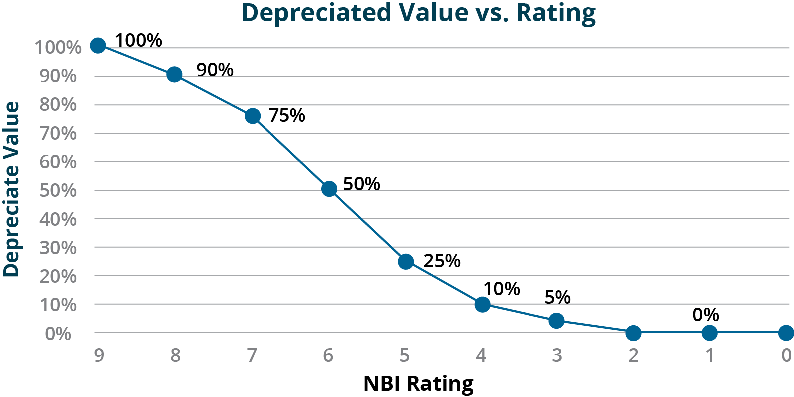
The Kentucky Transportation Cabinet (KYTC) uses a condition-based depreciation approach for valuing assets in its TAMP (37). For bridges KYTC bases depreciation on the NBI condition ratings for the deck, superstructure, and substructure of each bridge. For each value in the NBI scale KYTC has established an equivalent percent of depreciated value, as shown in Figure 6-4.

In Table 6-2 this depreciated value is mapped to an effective remaining service life using KYTC’s assumed useful life of 75 years for a new bridge. The remaining asset life can be substituted into the equation shown in Example 6-1 to calculate depreciation in dollars as a function of condition. The table shows an example of the calculations for a component with an initial value of $10 million.
Table 6-3. Effective Remaining Life and Depreciation Calculations by Condition Rating
| Condition Rating | Depreciated Value (see Figure 6-4) | Effective Remaining Useful Life (years) | Depreciation Given Initial Value of $10M ($M) | Current Value Given Initial Value of $10M ($M) |
|---|---|---|---|---|
| 9 | 100% | 75.00 | 0.0 | 10.0 |
| 8 | 90% | 67.50 | 1.0 | 9.0 |
| 7 | 75% | 56.25 | 2.5 | 7.5 |
| 6 | 50% | 37.50 | 5.0 | 5.0 |
| 5 | 25% | 18.75 | 7.5 | 2.5 |
| 4 | 10% | 7.50 | 9.0 | 1.0 |
| 3 | 5% | 3.75 | 9.5 | 0.5 |
| 2 | 0% | 0.00 | 10.0 | 0.0 |
| 1 | 0% | 0.00 | 10.0 | 0.0 |
A highway agency is interested in analyzing the pattern of consumption of benefits for pavement. Pavement management staff model the benefit of a pavement section as providing mobility for road users, reducing travel time and operating costs relative to an alternative of using other roads in the event the pavement section was out of service. Over time the use of the pavement increases, in theory yielding greater benefits. However, as the pavement ages roughness increases, reducing benefits obtained from the pavement.
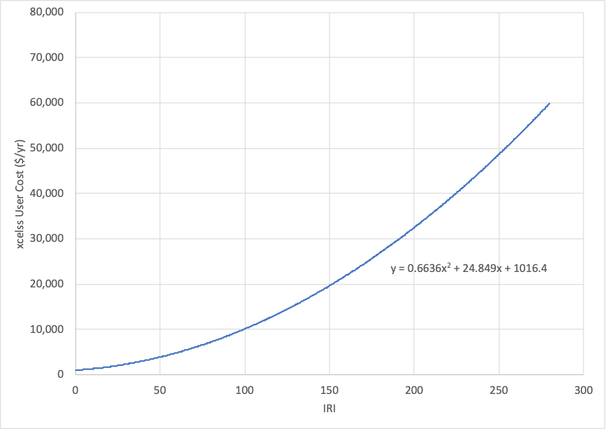
To model these effects the agency staff utilize the model of pavement user costs detailed in NCHRP Report 866 (38). Using the model provided with this report they predict the excess user costs for different representative pavement sections. Figure 6-5 shows the excess user cost as a function of IRI for a 1-mile urban principal arterial with daily traffic of 1,000 vehicles calculated using this model.
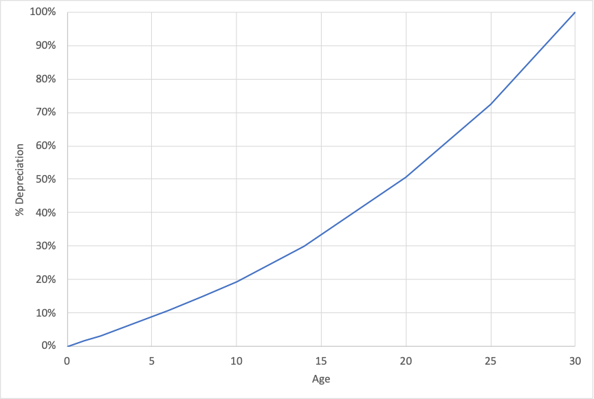
The staff use relationships obtained using the NCHRP report to estimate the benefits realized from a pavement section over time. This is then used to estimate the depreciation curve for pavement. Figure 6-6 shows an example curve for a one-mile section with 1,000 daily vehicles, assuming 5% annual growth in traffic.

