Depreciation is defined as “the loss of value of an asset or class of assets, as they age.” (1). Depreciation represents the consumption of capital, or the consumption of the benefits of an asset. From an accounting perspective, the depreciation calculated over some period measures how much value of an asset has been “used up.” From the perspective of an asset manager, depreciation is a measure of how much closer an asset has moved toward the end of its useful life.
Depreciation is calculated when it is necessary to adjust an asset’s value over time. If an asset’s value is based on the initial cost of constructing or purchasing the asset, the value at a later point should be depreciated. If one is using a market or economic perspective to establish value, then it may not be necessary to calculate depreciation. In such cases, depreciation may need to be calculated if adjusting a prior calculation of asset value. However, it is preferable to simply revalue the asset by repeating the calculation of value performed as described in Chapter 4.
Depreciation is closely related to deterioration, or decline in the physical condition of an asset. Generally speaking, as an asset ages, its benefits are consumed and it deteriorates. However, the consumption of benefits (as measured by depreciation) and the decline in condition (as measured by deterioration) often occur at different rates. For example, in accounting it is common to assume accelerated depreciation, in which asset value is assumed to decline more rapidly for a new asset than an older one.
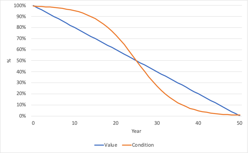
Below is an example illustrating how a deterioration curve can be used to calculate depreciation. Here value and condition are both depicted as a percentage of the value for a new asset. In this case, depreciation is assumed to be linear. Thus, the value of the asset decreases linearly from its initial value to its residual value. Condition of the asset follows an s-shaped curve (a logistic curve), in which the condition declines gradually near the beginning and end of an asset’s life, and more rapidly in the middle of its life. In this example it is further assumed that the asset is operated in the same manner over its entire life. Thus, the fact that physical conditions are declining more rapidly or slowly at different points in its life is immaterial: the key question is that of the remaining life of asset, which may need to be revised based on the asset’s condition. This example is representative of assets such as pieces of equipment that remain in service until the end of their life, and are used in the same manner generating the same benefits as long as they are safe to operate.
When the benefits derived from an asset depend upon its physical condition, the situation is different. In these cases, depreciation may be directly tied to deterioration, and therefore age is no longer an appropriate approximation. For example, for rail cars one might consider that as a vehicle ages riders suffer greater discomfort from riding on the vehicle and are more prone to experiencing delays in service. For pavement, user costs increase as pavement condition worsens. In such cases, the pattern of depreciation may better match the pattern of deterioration and a condition-based depreciation approach is best suited.
Depreciation may incorporate other factors beyond deterioration, as well. One key issue is technical obsolescence. Estimates of asset useful life typically incorporate assumptions concerning obsolescence, but this is not a factor incorporated into deterioration estimates. Assets can become obsolete due to technological or functional factors. For instance, a traffic controller may be in excellent physical condition, but would be considered to be obsolete if it no longer met industry technical standards and/or if it was no longer feasible to obtain replacement parts for the asset. Likewise, a bridge may be considered obsolete if designed to outdated functional standards for clearances and load carrying capacity. Typically once an asset is obsolete it assumed to be fully depreciated.
Another complicating factor that may be considered in calculating depreciation is the level of use of an asset, which may change either as a function of time, asset condition, or other factors. For example, a transit agency may use an older vehicle in poor condition less, utilizing newer, more reliable vehicles instead where feasible. On the other hand, for highway assets, traffic may continue to increase over time regardless of the condition of the asset, suggesting accelerating rather than decelerating depreciation.
Determining the various benefits an asset yields and how these vary over time can be an involved process. However, for most applications various simplifying assumptions are made to reduce the complexity. The different approaches can be grouped into three basic types, representing different levels of complexity in the calculations and data requirements. Table 6-1 lists the basic types of deprecation approaches and summarizes the strengths and weaknesses of each approach.
Table 6-1. Approaches for Calculating Depreciation
| Approach | Description | Strengths | Weaknesses |
|---|---|---|---|
| Actual Age | Depreciation increases linearly as a function of actual age | Straight-forward to calculate for new assets Requires few additional assumptions | Historic data may not be available, particularly for asset components Data on last treatment may be needed to establish age |
| Condition-Based | Depreciation increases linearly as a function of age adjusted for condition | Accommodates consideration of a wide range of treatments Can be calculated without historic data Supports evaluation of treatment selection and timing for TAM | Requires collecting condition data, frequently at a component level Can be a challenge to relate condition to remaining life, particularly for assets in very good or very poor condition |
| Non-Linear Benefit Consumption | Pattern of depreciation is determined based on a tailored analysis of how benefits are consumed | Flexible approach Consistent with U.S. and international accounting standards Best approach for matching actual pattern of use of an asset | Involves supplemental analysis Results may be dependent on parameters such as traffic growth and discount rate which are outside the control of an asset manager |
The simplest approach to calculating depreciation is to assume “straight-line depreciation” based on asset age. In this approach, one establishes the age of an asset or asset component, and then assumes depreciation increases in a linear fashion over the asset’s useful life. Thus, the value of the asset is presumed to decline by a constant value each year, dropping from the initial value to the end-of-life residual value. The virtue of this approach is its simplicity. When given an initial value, residual value, useful life, and asset age one can quickly determine asset value without any additional assumptions.
For any asset where very limited data exist, this relatively simple approach provides the asset manager with a functional method to determine a depreciation value. This approach can be applied to assets for which limited inventory data are available, assuming a distribution of asset age based on a model or sample data. Such approaches can be used to estimate value for assets such as signs and drainage structures which are numerous, but for which agencies may not have comprehensive data. Also, depreciating based on age can help address cases where an older asset becomes technically obsolete regardless of its physical condition.
In many cases, simply basing depreciation on an asset’s age can be too simple for supporting TAM applications. Often the age of an asset is a poor predictor of its remaining life, particularly if treatments have been performed to extend its life. Including effects of treatments further complicates the calculation. Replacing an asset resets its age, but what is the impact of a preservation action or a rehabilitation action? Further, many treatments impact one component of a complex asset but not others (e.g., the deck of a bridge but not the substructure; or the propulsion system of a rail car but not the carriage). Thus, when considering treatments short of replacement, one may need to track age and treatment effects at a component level.
A further complication is that it is frequently difficult to determine the age of an asset, particularly at a component level. We may know that a given section of a highway was constructed 40 years ago, but that does not necessarily imply that the pavement surface of the highway is 40 years old, let alone accompanying signs, guardrails, and other supporting assets.
Asset managers routinely contend with these challenges when modeling assets in their asset management systems. For some asset classes, such as guardrails and ITS, the asset’s age remains the best predictor of how the asset will perform and what treatments may be needed. Technical obsolescence can be a major factor for assets such as ITS devices. In some cases, there may be changes in standards or technical requirements that render assets obsolete sooner than would have been expected based upon their age. For complex assets, such as roads, bridges and facilities, information on asset age is supplemented with measurements of condition to better support TAM.
Where age data are unavailable or do not provide a reliable estimate of the remaining life of an asset, it may be preferable to base depreciation on an asset’s physical condition. If available, information on an asset’s condition can be used to obtain an improved estimate of the remaining life of an asset, and by extension, its effective age. There are many different approaches for utilizing condition data, but the approach that is recommended here can be generalized as follows: one obtains a revised, effective age for an asset using the available condition data, and then can proceed with asset valuation using this new effective age rather than actual asset age.
Note that the conversion of condition to age may involve a simple conversion and/or additional business rules. For instance, one may define a mapping of condition to percentage of life remaining, but decide to base the effective age on the actual age if the age or condition reach some threshold value. The key points are that condition is used in some manner to refine the estimate of an asset or asset component’s remaining life, and depreciation is assumed to proceed linearly once an age is established.
An alternative approach utilizing condition is to base depreciation strictly on condition without translating condition into an effective age. With this alternative approach it is implicitly assumed that benefits are consumed in proportion to the decline in condition, (which is typically a non-linear function). This approach is not recommended unless supported by additional analysis to verify the assumption that benefit consumption and condition change in direct proportion to one another. Where this alternative approach is used, it falls in the domain of a non-linear benefit consumption pattern as described further in the next section.
The basic advantage of calculating an effective age is that it leverages available condition data to provide a better estimate of how much of an asset’s value actually remains. Also, with this approach one can incorporate effects of treatments in the calculation of current value without specific knowledge of the treatment history of an asset. On the other hand, calculating effective age is practical only if condition data are actually available. Frequently, asset managers face limits to the available data, so in many cases, they rely on results of visual inspections and/or measurements of surface distresses. Needless to say, there are many challenges in relating the available data to the remaining service life of an asset.
With both of the general approaches described above, benefit consumption is assumed to be linear with respect to asset age (either actual or effective). A linear model should be assumed for depreciation unless there is evidence to suggest otherwise. This approach follows the maxim often attributed to Albert Einstein: “Everything should be made as simple as possible, but not simpler.”
However, in some cases an asset manager may have reason to believe that an asset will depreciate in some other manner. The final group of depreciation approaches encompasses the set for which benefits are consumed in a non-linear manner. When using a non-linear approach, one must carefully consider what benefits are being modeled and how these are actually consumed. Once a pattern is established, it can be mapped to actual or effective asset age to calculate depreciation.
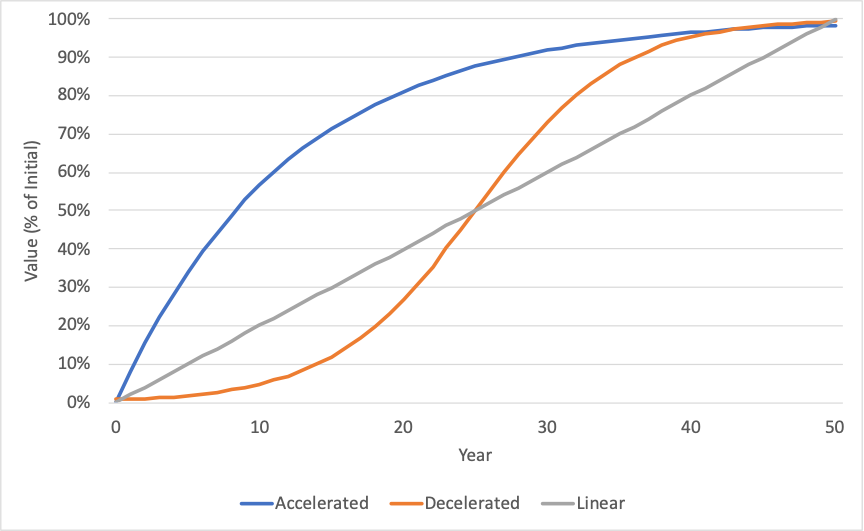
Figure 6-2 provides an example illustrating the impact of different non-linear benefit consumption patterns. In both cases depreciation is shown as a percentage of an asset’s initial value with an assumed residual value of 0. Here the asset is assumed to have a useful life of 50 years.
In the case of the lower, concave curve depreciation is accelerated: the asset loses more of its value initially and less towards the end of its useful life. This curve was developed using an exponential function of the following form:
\begin{align*} D(t) &= (V(t_0) - RV) * (1 - (1 - r)^t) \end{align*}
where:
This pattern of depreciation is applicable if the use of an asset decreases as it ages, such as in the example of a revenue vehicle described above. It can be used to support certain traditional accounting approaches, including “declining balance depreciation” and “double declining balance depreciation” as described in by Dojutrek, et. al. (35). To use declining balance depreciation, one would set r to be equal to \frac{1}{N} where N is the useful life of the asset. To use double declining depreciation, one would set r to be \frac{2}{N}.
For the upper curve depreciation is decelerated: the asset loses less of its value initially, but then depreciation accelerates towards the end of the asset’s useful life. This curve was developed using a logistic function of the following form:
\begin{align*} D(t) &= \frac{V(t_0) - RV}{1 + e^{c_1 + c_2t}} \end{align*}
where c_1 and c_2 are constants.
This functional form may be applicable in cases where use of an asset is increasing over time, and/or where an asset’s benefits are proportional to asset condition. For instance, in the case of pavement, asset value may be represented using a condition index that is inversely proportional to road user costs.
The approach of defining a customized, non-linear depreciation curve to match the pattern of consumption of an asset’s benefits is flexible, and consistent with U.S. and international accounting standards. Also, it is highly compatible with the economic perspective of asset value. If one has calculated initial asset value based on economic value, then establishing a specific pattern of depreciation can be performed using the same data compiled to calculate initial value.
The challenge with this approach is that it can be time consuming to perform the analysis required to establish an alternative benefit consumption pattern. Also, the results may hinge on assumptions outside the control of the asset manager, such as traffic growth. An asset manager may ask whether “the juice is worth the squeeze” before undertaking the additional analysis required for this approach.
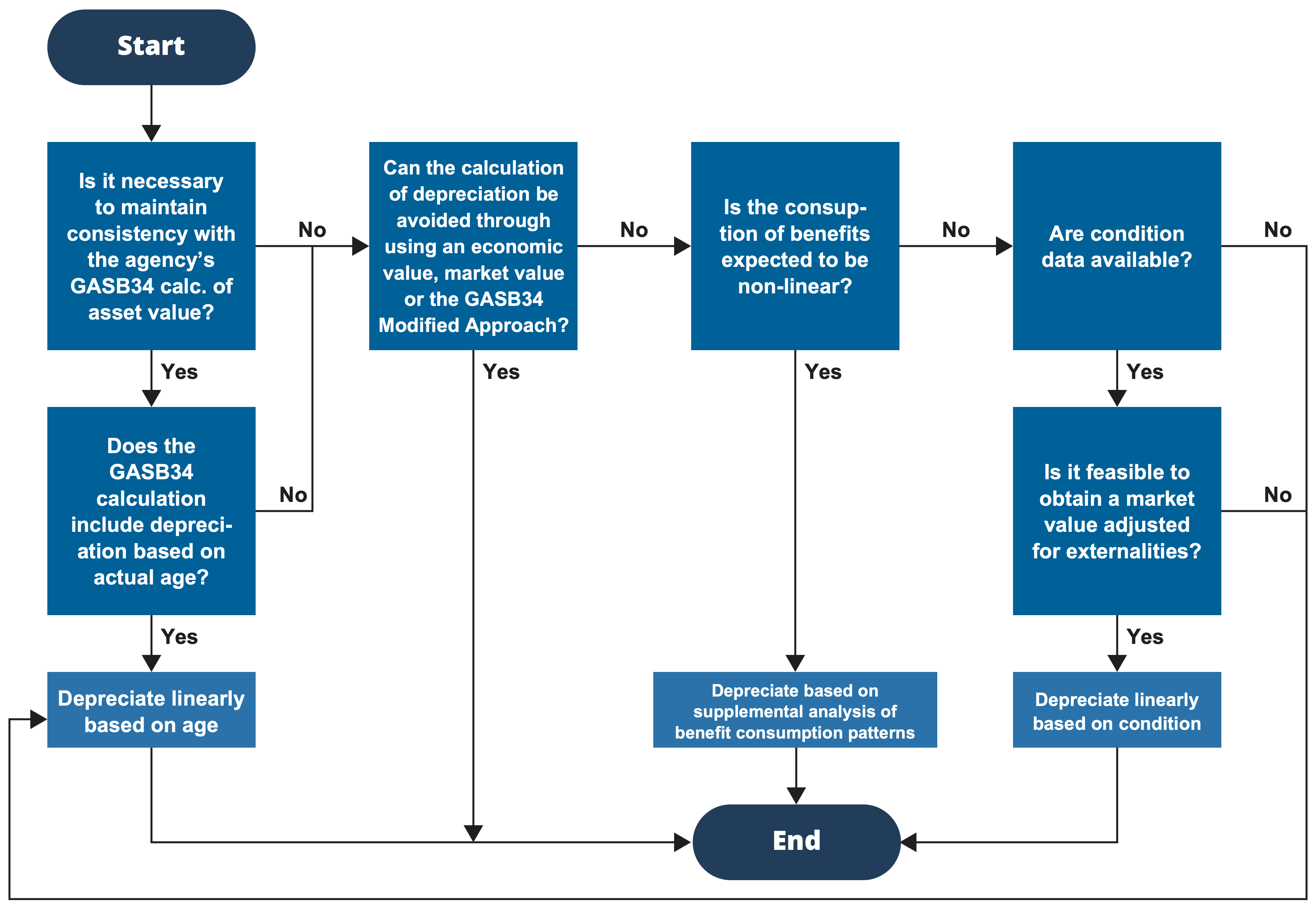
While all of the approaches for calculating depreciation are valid, various approaches are preferable for certain TAM applications and depending on what data one has available. Figure 6-3 is a flowchart recommending an approach for calculating depreciation. Following the chart, results in a recommendation to either avoid the depreciation calculation entirely, depreciate linearly based on actual age, depreciate linearly using a condition-based approach, or perform supplemental analysis to establish the depreciation pattern if there is reason to believe it is non-linear. The basic logic reflected in the flowchart is:
- In certain cases, it is not necessary to calculate depreciation. If one is using the GASB 34 modified approach a cost to maintain is calculated using an organization’s management systems, but depreciation is not specifically calculated. In cases where one requires the current value of the asset and obtains this from the calculation of initial value – e.g., in the case of economic or market value – then additional calculation of depreciation is not needed. In all other cases, depreciation should be calculated.
- Linear depreciation based on actual age should be used as the basis for depreciation if this approach was used for financial reporting based on GASB 34 and the agency seeks to maintain consistency with its financial reporting. GASB 34 does not require that agencies assume linear depreciation based on asset age, but this is the approach that is almost invariably used except in cases where an agency uses the GASB 34 modified approach.
- Depreciation is important when using the replacement cost method because it indicates asset condition. Replacement cost alone only provides the “worst-case” estimate of asset cost. By accounting for depreciation, agencies demonstrate a commitment to maintaining the asset and avoiding the single, large replacement cost at the end of the asset’s life.
- In cases where depreciation is calculated and consistency with the approach used for financial reporting is not strictly required, then one must next ask whether there is reason to believe the pattern of benefit consumption may be non-linear. If this is the case, then further analysis will be required to establish the specific depreciation approach.
- Otherwise, one should use condition data to establish effective age if condition data are available and provide a meaningful estimate of the remaining life of an asset. Actual age should be used if condition data are unavailable, or if asset condition does not help predict remaining life (e.g., for assets that tend to be replaced due to obsolescence).
Note that based on the flow chart does there may arise a case where it is preferable to base depreciation on condition, but condition data are unavailable. In the flow chart one is directed to use an age-based approach in this case. However, this raises a broader question of what data an agency collects on its assets and how to assess data needs. NCHRP Report 956 (17), Chapter 7 of the AASHTO TAM Guide, Second Edition (5), and Chapter 8.5 of the AASHTO TAM Guide, First Edition (36) are all valuable references for further discussion of this topic.


