In this example, a highway agency in the Northern U.S., labeled “The Northern Agency,” is interested in calculating asset value and related measures to report for highway-related assets in its TAMP. Note, this example is adapted from tests with two different agencies, and is not intended to be representative of any actual agency.
Following the process outlined in Section 2, the agency first establishes that its goal is to establish overall value and related measures for three asset classes: pavement; structures (including bridges and bridge-length culverts); and buildings. The agency has data at the asset-level for each asset class. For pavement and structures, the agency has detailed condition data. For buildings, the agency has only summary inventory data, but its facility division has separately established insurance values representing the amount each building is insured for in the event of a catastrophic event, independent of the value of land or the equipment in each building.
For their structures, the agency decides that asset value should be computed at a component level, given that different structure components have different useful lives and condition data are available to support the calculation. Bridges are represented using three components: the bridge deck, superstructure and substructure. Bridge-length culverts are represented as a single component.

The following subsections describe the approach used for Steps 2 to 4 of the asset value calculation by asset class, followed by a summary of the results.
Pavement
Using the flow chart in Chapter 4 the agency decides that initial value for pavement should be based on replacement cost, given there is no need to maintain consistency with the approach used for financial reporting (based on historic costs), no specific need to calculate value of the asset class to society (which would suggest a need for calculating economic value), nor is there a market value that may be readily determined as an alternative.
Next, the agency reviews its treatment strategy for pavements. Initial construction of pavement is estimated to cost $1.4 million per lane mile. When a pavement section reaches the end of its useful life it is reconstructed at a cost of approximately $1 million per lane mile, restoring it to “like new” condition. Various treatments are performed over a pavement’s life, and their effects are reflected in the Pavement Condition Index (PCI) at any given time. PCI is an agency-specific measure of pavement condition. It combines different pavement distresses into a scale from 0% (worst condition) to 100% (best condition).
Given their use of the replacement cost approach to calculate initial value and PCI to capture condition, the agency determines it is not necessary to incorporate other treatments in the calculation of asset value besides pavement construction and reconstruction. Based on the agency’s life cycle strategy, the pavement is deemed to reach the end of its useful life when its PCI is reaches a value of 25%, which typically occurs at an age of approximately 25 years, as depicted in the deterioration curve shown in Figure 9-2. The pavement assets’ residual value is estimated to be $0.4 million per lane mile, equal to the difference in cost between initial construction and reconstruction.

Then, the agency considers how to calculate depreciation. Reviewing the flow chart in Chapter 6, the agency decides to use a condition-based approach for calculating depreciation. The PCI of a pavement section estimates the effective life remaining where condition data are available. Where data are unavailable, the asset’s actual age is used. Figure 9-3 summarizes the distribution of pavement condition, depicting the percentage of pavement lane miles for each effective age from zero to over 24. Most of the assets have an effective age of under five years.

The agency uses the above information to calculate the value of its pavement. Initial value is approximately $30.8 billion (22,000 lane miles x $1.4 million per lane mile). For each section, depreciation is calculated based on the effective age using the depreciation formula for the condition-based approach, provided in Chapter 6. The result is that current pavement value is calculated as $26.0 billion with annual depreciation equal to $876 million. Annual depreciation is calculated by aging each pavement section by an additional year and noting the resulting change in value.
Structures
After completing the pavement valuation, the agency walks through the same process outlined above for structures, considering each of the bridge components defined. As in the case of pavement, the agency decides that initial value should be based on replacement cost.
The agency next reviews its treatment strategy for bridges and bridge-length culverts. The construction of a bridge or culvert costs approximately $280 per square foot of deck area. Replacing a structure has a similar cost. The approximate costs for replacing bridge decks, superstructures and substructures are established based on a pro-rated share of the total bridge replacement cost, considering the relative costs of replacing the component parts. Based on these historic costs, the bridge deck replacement is estimated to be 25% of the value of the bridge, the superstructure is estimated to be 40% of the value, and the substructure is estimated to be 35% of the value. Various treatments are performed over the life of a component, and their effects are reflected in the component conditions ratings. These are measured on the 0 to 9 scale defined for the NBI. When a component has reached the end of its useful life either the component is replaced or the entire structure may be replaced.
Given the incorporation of the component condition ratings into the NBI, the agency determines it is not necessary to include any treatments in the calculation of asset value besides initial construction and component or bridge replacement. Based on the agency’s life cycle strategy, a bridge deck is deemed to be at the end of its useful life when it has a rating of 4 or less on the NBI scale. For the superstructure, substructure and culverts, the component is deemed to be at the end of its useful life when it has a rating of 3 or less. Figure 9-4 illustrates the agency’s deterioration curves depicting the effective age of a component as a function of its condition rating. The agency developed these curves for use in their management systems based on an analysis of historic bridge inspection data. Three curves are shown in the figure: one for decks; a second used for both superstructure and substructure; and a third curve for culverts.
The agency further establishes that a portion of its bridges are built to outdated functional standards for load capacity and clearances. These bridges are deemed to be at the end of their useful life regardless of their physical condition. Thus, these bridges are treated as fully depreciated when calculating their asset value.

The agency then considers how to calculate depreciation. As in the case of pavement assets, the agency decides to use a condition-based approach. The NBI component rating is used to establish effective age. Figure 9-5 summarizes the distribution of conditions, depicting the percentage of each component in each condition rating (exempting functionally obsolete structures).

Lastly, the agency uses the approach described above to calculate value. Initial value is approximately $14.0 billion (50 million square feet x $280 per square foot). The calculations of current value are made by component, grouping all of the components of a given rating together (and exempting the obsolete bridges). For each rating group, effective age is estimated using the agency’s deterioration curves, and then depreciation is calculated using the depreciation formula provided for the condition-based approach in Chapter 6. The result is a current structure value of $8.8 billion. With annual depreciation equal to $193 million; this can be calculated by aging each group by an additional year and noting the resulting change in value.
Buildings
For its buildings, the agency has more limited condition data than it has for pavement and structures. However, as noted above, in addition to its data on the building inventory, the agency has data on the insured value of each of its buildings. The agency decides to use this insured value as a proxy for market value. The agency thereby establishes that the insured values of its buildings totals $0.9 billion.
The agency establishes the cost to replace all of its buildings would be approximately $1.2 billion, and that buildings are estimated to have a useful life of 60 years. The agency determines that an age-based approach should be used for depreciation if it is necessary to further depreciate the market value. Annual depreciation is estimated at approximately $20 million (equal to the replacement cost of $1.2 billion divided by the useful life of 60 years).
Results Summary
Table 9-1 summarizes the results of the asset value calculation. For each asset class, it shows the replacement cost, current value, ACR, and annual depreciation. The total replacement cost for all of the Northern Agency’s highway assets totals $46 billion. Considering the effects of depreciation, the current value of the inventory is $35.7 billion, resulting in an ACR of 0.78. Note there is no specific target value for ACR, but ideally this measure is maintained or increased over time. Absent investment to increase asset value, the inventory is expected to depreciate approximately $1.1 billion per year. This estimate of annual depreciation can be used as an estimate of the Cost to Maintain Value, though as described in Chapter 7 this cost should ideally be calculated using an agency’s asset management systems.
Table 9-1. Summary Results for the Northern Agency
| Asset Class | Subclass | Replacement Cost ($ billion) | Current Value ($ billion) | Asset Consumption Ratio (ACR) | Annual Depreciation |
|---|---|---|---|---|---|
| Pavement | 30.8 | 26.0 | 0.84 | 876 | |
| Structures | Bridges | 13.4 | 8.5 | 0.63 | 187 |
| Culverts | 0.6 | 0.3 | 0.61 | 6 | |
| Subtotal | 14.0 | 8.8 | 0.63 | 193 | |
| Buildings | 1.2 | 0.9 | 0.75 | 20 | |
| Total | 46.0 | 35.7 | 0.78 | 1,089 | |
This example presents a transit agency, located in the Western U.S., termed “The Western Agency.” The agency operates three different transit modes: buses; paratransit vehicles (also called “cutaways”); and a Light Rail Transit (LRT) system. The agency’s asset hierarchy is summarized in Figure 9-6. Major asset classes include revenue vehicles, equipment (service vehicles), facilities and infrastructure. Each of these asset classes consists multiple subclasses. The infrastructure asset class includes the largest number of subclasses. In addition to LRT track, which may be either tangent (straight) or curved, this class includes bridges, special trackwork (grade crossings and switches), and power assets (catenary wire segments, relay cases, and substations).

Previously the Western Agency reported asset value in its TAMP based on the historic cost of asset acquisition or construction. This approach was used to maintain consistency with the agency’s reporting of asset value in its financial statements. As part of the previous effort, the agency collected data on the historic cost and year of purchase or construction for each of the asset classes and subclasses in the TAMP. For revenue vehicles, equipment and facilities costs are tracked at the asset level. For infrastructure assets, costs are tracked by asset subclass, grouping all assets of a given subclass built at a similar time.
For its next TAMP, the agency seeks to report value based on current replacement cost rather than historic cost, as current replacement cost is more closely tied to the cost of rehabilitating and replacing assets. However, for now the agency intends to include both the historic cost of its assets and the current depreciated replacement cost to facilitate comparison with the values in its prior TAMP.
The following subsections describe the approach the agency used for the asset value calculation, followed by a summary of the results. The asset classes are combined into two groups in the discussion: vehicles, which includes revenue vehicle and equipment; and fixed assets, including facilities and infrastructure.
Revenue Vehicles and Equipment (Service Vehicles)
As described above, the agency seeks to establish initial value based on current replacement cost. The agency estimates this initial value by adjusting the historic cost paid for each vehicle for inflation. The agency estimates the annual inflation rate for revenue and service vehicles has historically been approximately 1.6 percent.
The agency next reviews its treatment strategy for vehicles. The agency has established the useful life for its vehicles by vehicle type assuming that planned maintenance and rehabilitation activities are performed on a vehicle over its useful life. The useful life shown in Table 9-2 is estimated based on historical asset performance. At the end of a vehicle’s useful life the vehicle is replaced with a new vehicle. Since vehicle treatments are included within the useful life estimates, the agency establishes that the only treatment explicitly modeled in the asset value calculation should be the initial purchase of the vehicle. While the agency auctions used assets at the end of their useful life, the value received is negligible, so for the sake of this analysis, they assume a residual value of $0. To depreciate vehicle asset value the agency elects to use an age-based approach. The depreciation calculation is made separately for each vehicle.
Table 9-2. Useful Life for Vehicles
| Asset Class | Subclass | Useful Life (years) |
|---|---|---|
| Revenue Vehicles | Buses | 14 |
| Light Rail Vehicles | 40 | |
| Paratransit Vehicles | 10 | |
| Equipment (Service Vehicles) | Automobiles | 8 |
| Steel Wheeled Vehicles | 25 | |
| Trucks and Other Rubber-Tired Vehicles | 14 |
Facilities and Infrastructure
As in the case of vehicles, the agency seeks to establish initial value based on current replacement cost. The agency estimates this initial value by adjusting the historic construction costs of each asset for inflation. The agency estimates the annual inflation rate for construction has been approximately 3.0 percent over the facilities’ lifespan.
Next, the agency reviews its treatment strategies for fixed assets. For these assets, the agency periodically measures asset conditions using the five-point condition scale established by FTA. Using this scale, condition ranges from 1 (worst condition) to 5 (best condition). If an asset has a condition of 2 or less it is deemed to be not in good repair and beyond its useful life. Useful lives are established by asset class, as shown in Table 9-3. When an asset has reached the end of its useful life it is replaced. The agency performs different treatments on an individual asset over its life, but these are reflected in its condition score. Given the availability of condition data, the agency establishes that the only treatment explicitly modeled in the asset value calculation is the asset construction. The agency further assumes that the residual value of an asset at the end of its life is $0.
Table 9-3. Useful Life for Fixed Assets
| Asset Class | Subclass | Useful Life (years) |
|---|---|---|
| Facilities | Administrative | 60 |
| Maintenance | ||
| Public Facilities | ||
| Infrastructure | LRT Track - Tangent | 35 |
| LRT Track - Curved | 30 | |
| LRT Bridges | 70 | |
| Grade Crossings | 15 | |
| Switches | 25 | |
| Catenary Wire Segments | 25 | |
| Relay Cases | 50 | |
| Substations | 25 |
To depreciate asset value the agency elects to use condition-based approach assuming that the change in condition is proportional to age. The effective age of an asset as a function of condition is modeled as follows:
E(c) = \frac{UL (5-c)}{(5-2)}
where E(c) is the useful life for a given condition c and UL is the useful life. The denominator is represented by the condition rating at the end of the asset’s useful life subtracted from the highest possible condition rating. With this approach, the effective life of an asset is 0 if its condition is rated as a 5 and is equal to its total useful life if the rating is 2 and it is fully depreciated.
Results Summary
Table 9-4 summarizes the results of the asset value calculation. For each asset class and subclass, it displays the historic cost, replacement cost, current value, ACR and annual depreciation. The table shows that the historic cost of the agency’s assets is $3.1 billion. Adjusting the historic costs for inflation, the current replacement cost of the asset inventory is estimated to be approximately $4.5 billion. The current value, which incorporates depreciation, is approximately $2.7 billion. The ACR for the agency’s asset inventory is 0.60, equal to the current value divided by the replacement cost. Absent investment in the assets, the inventory is expected to depreciate approximately $123 million per year.
Table 9-4. Summary Results for the Western Agency
| Asset Class | Asset Subclass | Historic Cost ($M) | Replacement Cost ($M) | Current Value ($M) | Annual Depreciation ($M) | ACR |
|---|---|---|---|---|---|---|
| Revenue Vehicles | Bus | 456 | 498 | 298 | 34 | 0.60 |
| Light Rail Vehicle | 506 | 603 | 433 | 15 | 0.72 | |
| Paratransit | 25 | 26 | 17 | 3 | 0.65 | |
| Subtotal | 987 | 1,127 | 748 | 51 | 0.66 | |
| Equipment | Automobiles | 3 | 3 | 1 | 0 | 0.27 |
| Steel Wheeled Vehicles | 2 | 2 | 2 | 0 | 0.86 | |
| Trucks and Other Rubber-Tired Vehicles | 35 | 39 | 23 | 3 | 0.60 | |
| Subtotal | 40 | 44 | 26 | 3 | 0.59 | |
| Facilities | Administrative | 19 | 39 | 23 | 1 | 0.58 |
| Maintenance | 170 | 400 | 195 | 7 | 0.49 | |
| Public Facilities | 925 | 1,485 | 789 | 25 | 0.53 | |
| Subtotal | 1,114 | 1,924 | 1,007 | 32 | 0.52 | |
| Infrastructure | LRT Track - Tangent | 503 | 710 | 473 | 20 | 0.67 |
| LRT Track - Curved | 144 | 203 | 135 | 7 | 0.67 | |
| LRT Bridges | 190 | 268 | 161 | 3 | 0.60 | |
| Grade Crossings | 4 | 6 | 3 | 0 | 0.57 | |
| Switches | 4 | 5 | 3 | 0 | 0.50 | |
| Catenary Wire Segments | 35 | 50 | 26 | 2 | 0.53 | |
| Relay Cases | 65 | 87 | 70 | 2 | 0.80 | |
| Substations | 34 | 46 | 28 | 2 | 0.60 | |
| Subtotal | 980 | 1,374 | 899 | 37 | 0.65 | |
| Total | 3,121 | 4,469 | 2,680 | 123 | 0.60 | |
In this example, a state department of transportation in the Midwest, labeled the “Midwest DOT,” applies the economic value approach to quantify benefits realized by users of the state’s primary roadway network. For this example, the state’s primary roadway network is defined as all state-owned Interstates, primary arterials, minor arterials, and major collectors. This example follows the economic approach described in Chapter 4 to estimate the benefits of the primary roadway system. The example provides a better understanding of the value generated by the roadways for direct users and society as a whole. This example shows how state DOTs can estimate the value assets provide to users as compared to the replacement value method, which focuses on what those assets cost.
Application of Economic Value Approach
This case study includes the following basic steps:
- First, traffic data were collected on the Midwest DOT’s primary roadway network. This included all Interstates, principal arterials, minor arterials, and major collectors.
- Second, fatality and serious injury crash rates were collected. These data are maintained by the Midwest DOT and available at the state level.
- Third, emissions rates for the state were collected from the Environmental Protection Agency (EPA) MOVES model. A representative county was selected to generate emissions rates specific to the state.
- Fourth, these data were used to calculate user benefits for the value of travel time, vehicle operating costs, safety, and emissions.
- Fifth, the research team examined the model to interpret the results and found that users of the roadway network experience a much higher monetary value of benefits than the Midwest DOT reports in its TAMP as the replacement costs of the system.
These steps are detailed in the following subsections. A theoretical discussion of the approach is presented at the end of the case study.
Data Collection
The Midwest DOT reports traffic data annually to the Federal Highway Administration (FHWA) as part of its Highway Performance Monitoring System (HPMS) reporting requirements. This data provides a convenient summary of traffic data that can be collected for any state DOT. While 2020 HPMS data was available, this example referenced 2019 HPMS data to avoid any distortions due to restrictions and changed habits during the COVID-19 pandemic. This is consistent with 2021 USDOT guidance for federal discretionary grants, which noted that 2019 traffic data should be used rather than non-representative 2020 data (48).
The analysis utilized the following HPMS variables that were provided by the Midwest DOT:
- Route_ID – This variable is assigned to each individual roadway segment. This identification number is alpha-numeric and contains information on roadway direction, type, and location.
- Section_Length – This variable refers to the length, in miles, of each identified roadway segment. This variable was used, in part, to calculate vehicle-miles traveled (VMT) and vehicle-hours traveled (VHT). These two variables were the basis for estimating all benefits categories included in the analysis.
- F_System – This variable indicates the classification of the system and is broken into seven different types. Segments classified as 1, 3, 4, and 5 were isolated as those correspond with Interstates, principal arterials (other), minor arterials, and major collectors, respectively. Roadways classified as 2, 6 and 7—principal arterials (other freeways and expressways), minor collectors, and local roads, respectively—were not included in the analysis because they are not part of the principal roadway system and did not have a significant number of observations in the dataset.
- Facility_Type – This variable refers to the operational characteristic of the roadway. This variable is important to account for the correct mileage and average annual daily traffic (AADT). Most Interstate segments and many principle arterial segments are separated directionally. The codes used for this variable are as follow:
- 1 – One-way roadway
- 2 – Two-way roadway
- 3 – Couplet
- 4 – Ramp
- 5 – Non-mainline
- 6 – Non-inventory direction
- 7 – Planned/unbuilt
In the HPMS database, many separated Interstates and principal arterials are reported as bi-directional AADT for each separated direction of roadway, so the same bi-directional AADT is reported as Facility_Type 1 in the eastbound direction of a roadway and as Facility_Type 6 in the westbound direction. In order to avoid double-counting of AADT, roadway segments classified as “Non-inventory direction,” or Facility_Type 6, were excluded from this analysis.
- Ownership – This variable indicates the entity that has legal ownership of a roadway and is typically used for apportionment, administrative, legislative, analytical, and national highway database purposes and in cost allocation studies. This example only considers segments with Ownership code 1, which refers to roadways owned by the State DOT.
- Urban_Codes – This variable refers to the U.S. Census Urban Area Code and is used for the querying and analyzing data by the unique identification of a state’s urbanized areas and generically by small urban or rural areas. For this example, the values of urban and rural travel are separated. All segments coded as 99998 or 99999 were considered rural and all others were considered urban.
- AADT – This variable provides the bi-directional annual average daily traffic counts of all vehicles and trucks traveling on the roadway. This variable was used, in part, to calculate VMT and VHT. As discussed above, the “Facility_Type” variable was used in combination with AADT to ensure that bi-directional AADT is not “double counted” in the case of divided or separated roadways.
- AADT_Combination – This variable provides the bi-directional annual average daily traffic counts for combination trucks. Trucks have different operating costs, emission rates, and values of time, so these vehicles are treated separately from passenger vehicles in the analysis. This variable was used, in part, to calculate VMT and VHT as discussed further below.
- AADT_Single_Unit – This variable provides the bi-directional annual average daily traffic counts for single-unit trucks. Trucks have different operating costs and emission rates, and their value of time is calculated differently, so these vehicles are treated separately from passenger vehicles in this analysis. This variable was used, in part, to calculate VMT and VHT.
- Speed Limit – This variable reports the posted speed limit for every roadway segment. The Midwest DOT advised that due to negligible congestion statewide, the research team should use this as the measure for speed of travel. This variable was used, in part, to calculate the VHT of vehicles.
To summarize, roadway segments were sorted to include only those that are Midwest DOT-owned and classified as F_System type Interstate, principal arterial, minor arterial, or major collector. This calculation did not include minor collectors and local roads. Further, segments identified as non-inventory direction under the Facility_Type variable were excluded to prevent any double counting of AADT.
For each F_System type, VMT was calculated separately for urban and rural areas as identified by their Urban Codes. VMT was also calculated separately for passenger vehicles and trucks and aggregated along the criteria stated. The basic calculations for VMT are found below. Note that these calculations represent the VMT calculation for each individual segment. Total VMT is the sum of VMT for all roadway segments, calculated for Interstates, principal arterials, minor arterials, and major collectors and separately for urban and rural areas.
- Passenger Vehicle VMT = [Total Vehicles (AADT) – Total Trucks (AADT_Combination + AADT_Single_Unit)] * Section Length
- Truck VMT = [Total Trucks (AADT_Combination + AADT_Single_Unit)] * Section Length
VMT and speed limits were used to calculate VHT for the same roadway segment criteria. Total passenger vehicle and truck VHT were calculated by summing the VHT from each roadway segment. To calculate VHT, passenger vehicle and truck VMT for each segment was divided by the posted speed limit (in miles-per-hour), which was used as a proxy for average travel speed for this exercise. Typically, observed average travel speeds or VHT collected by the state or calculated using traffic modeling software would be preferable as a measure of vehicle speed, but in this instance the relevant roadways had sufficiently low to nonexistent congestion levels, so speed limit was used as an acceptable measure. The general calculation for passenger vehicle and truck VHT can be found below. Note that this is the VHT calculation for each individual segment. Total VHT would be the summed total of all the roadway segments.
- Passenger Vehicle VHT = Segment Passenger Vehicle VMT / Segment Speed Limit
- Truck VHT = Segment Truck VMT / Segment Speed Limit
User Cost Calculation
In the next step, monetary values were applied to the VMT and VHT aggregations to calculate the user benefits (or in this case, user costs) associated with willingness-to-pay for travel time, vehicle operating costs, safety, and emissions. This analysis utilized monetization parameters recommended per the United States Department of Transportation (USDOT) Benefit-Cost Analysis Guidance for Discretionary Grant Programs as of February 2021 (48).
Travel Time
USDOT guidance recommends a value of time for passengers and truck drivers of $17.90 and $30.80 per hour, respectively. Passenger vehicles are assumed to have 1.67 occupants and trucks are assumed to have one occupant. The basic calculations for the value of travel time for passenger vehicles and trucks used in this analysis can be found below:
- Total Value of Travel Time for Passenger Vehicles = $17.90 * 1.67 occupants * Total Passenger Vehicle VHT
- Total Value of Travel Time for Trucks = $30.80 * 1 occupant * Total Truck VHT
Vehicle Operating Cost
USDOT guidance recommends a per-mile vehicle operating cost of $0.43 for passenger vehicles and $0.93 for trucks. These values were applied directly to the VMT calculated for passenger vehicles and trucks. The basic calculations for the value of vehicle operating costs used in this analysis can be found below:
- Total Value of Passenger Vehicle Operating Costs = Total Passenger Vehicle VMT * $0.43
- Total Value of Truck Operating Costs = Total Truck VMT * $0.93
Safety
USDOT guidance recommends a monetized value of an averted fatality of $10,900,000 and a monetized value of an averted injury (of unknown severity) of $197,600. The Midwest DOT provided crash rates by severity and facility type for rural and urban areas in its Highway Safety Improvement Program (HSIP). These rates are reported as incident rates per hundred-million vehicle miles traveled (HMVMT). The basic calculations for the value of safety incidents used in this analysis can be found below:
Fatality Crashes
- Total Value of Passenger Vehicle Fatal Crashes = [Total Passenger Vehicle VMT / 10^6] * $10,900,000 * Fatal crash rate per HMVMT
- Total Value of Truck Fatal Crashes = [Total Truck VMT / 10^6] * $10,900,000 * Fatal crash rate per HMVMT
Injury Crashes
- Total Value of Passenger Vehicle Injury Crashes = [Total Passenger Vehicle VMT / 10^6] * $197,600 * Injury crash rate per HMVMT
- Total Value of Truck Injury Crashes = [Total Truck VMT / 10^6] * $197,600 * Injury crash rate per HMVMT
Emissions
USDOT recommends emissions valuations per metric ton of pollutant emitted by pollutant type and year. These monetized values are applied to pollutant quantities calculated using the EPA MOVES model for a representative county in the state. The MOVES model reports grams of pollutant emitted per mile driven. It has separate emissions rates for passenger vehicles and trucks, urban and rural roadways, and various speed bins which consider the different fuel efficiency experienced at different speeds. Below are the monetized values per metric ton of pollutant emitted by type and year.
Table 9-5. Cost per Metric Ton of Pollutant from the MOVES Model
| Emission Type | NOx | SO2 | PM2.5 | CD2 |
|---|---|---|---|---|
| 2020 | $15,700 | $40,400 | $729,300 | $50 |
| 2021 | $15,900 | $41,300 | $742,300 | $52 |
| 2022 | $16,100 | $42,100 | $755,500 | $53 |
| 2023 | $16,400 | $43,000 | $769,000 | $54 |
| 2024 | $16,600 | $43,900 | $782,700 | $55 |
| ... | ... | ... | ... | ... |
| 2050 | $18,000 | $48,200 | $852,700 | $84 |
The basic calculation for the value of emissions used in this analysis can be found below:
- Total Value of Passenger Vehicle Emissions = Total Passenger Vehicle VMT * [Grams of Pollutant Emitted by Type / 1000^2] * Monetary Value of Pollutant by Type
- Total Value of Truck Emissions = Total Truck VMT * [Grams of Pollutant Emitted by Type / 1000^2] * Monetary Value of Pollutant by Type
The value of emissions is dependent on the year in the analysis so annual emissions should be calculated for each year and applied to that specific year’s monetary value.
Analysis Period and Discounting
This exercise used a 20-year analysis period, which is consistent with USDOT BCA guidance. The beginning year for values was set at 2020 and concluded in 2039 to cover a 20-year period. In accordance with USDOT guidance, all monetized values were discounted at 7 percent with the exception of values related to carbon dioxide emissions, which were discounted at 3 percent. The general formula for calculating the discount rate can be found below:
- Discount Rate = 1 / [(1 + Discount Rate) ^ (Year of Analysis – Base Year of Analysis)]
Discounted benefits for each year were aggregated to calculate the discounted total benefits realized by the state’s primary roadway network over the analysis period. Because the benefits were calculated separately by F_System type and for urban and rural areas the total benefits can be viewed with added levels of granularity as needed.
Results of Economic Value Approach
This example reveals significant value in the state’s primary roadway network. Annual travel recorded in 2019 was projected with no assumed growth rate for each year of the analysis period. The value experienced by roadway users in Year 1 of the analysis was calculated at $13.2 billion. Over a 20-year time period this equates to $258.7 billion in undiscounted terms or $148.0 billion when discounted at 7 percent (3 percent for carbon dioxide emissions). The most significant drivers of value were travel time and vehicle operating costs, which were $5.7 billion and $6.1 billion (annually), respectively.
Table 9-6. Summary of the Midwest Agency’s Roadway Network Value
| User Cost Category | Single-Year Value ($B) | 20-Year Value Undiscounted ($B) | 20-Year Value Discounted at 7% (3% for CO2) ($B) |
|---|---|---|---|
| Travel Time | $5.74 | $114.79 | $65.06 |
| Vehicle Operating Costs | $6.05 | $121.02 | $68.59 |
| Traffic Safety | $0.71 | $14.10 | $7.99 |
| Emissions | $0.66 | $8.75 | $6.31 |
| Total | $13.16 | $258.66 | $147.95 |
The single year value experienced by the roadway is roughly half of the network’s total replacement value as reported in the Midwest DOT’s Transportation Asset Management Plan. This implies that after approximately two years of use the roadway network has already provided value to the public equal to the entire replacement cost of the network. A significant portion of the state’s travel occurs on the primary network and this is reflected in the significant value experienced by users.
Overall, the value realized in urban areas ($7.1 billion annually) is slightly greater than that realized in rural areas ($6.1 billion annually).
Table 9-7. Single Year Value for Urban and Rural Roads at the Midwest Agency.
| User Cost Category | Urban Single-Year Value ($B) | Rural Single-Year Value ($B) | Total Single-Year Value ($B) |
|---|---|---|---|
| Travel Time | $3.39 | $2.35 | $5.74 |
| Vehicle Operating Costs | $3.00 | $3.05 | $6.05 |
| Traffic Safety | $0.41 | $0.30 | $0.71 |
| Emissions | $0.25 | $0.41 | $0.66 |
| Total | $7.06 | $6.10 | $13.16 |
At the state level, Interstates account for $9.9 billion in annual value, principal arterials account for $3.2 billion, minor arterials account for $0.04 billion, and major collectors account for $0.02 billion. For the Interstate system alone, the rural annual value ($6.05 billion) exceeds urban annual value ($3.8 billion). Approximately 99 percent of the total value of Midwest DOT rural roadways is on the Interstates, with only $45 million of rural annual value coming from principal arterials, minor arterials, and major collectors. Principal arterials represent a much larger share of value in urban areas.
Overall, Interstates account for 75.0 percent of value, principal arterials account for 24.5 percent, and combined minor arterials and major collectors account for the remaining 0.5 percent.
Table 9-8. Single Year Value for Each Road Category at the Midwest Agency.
| User Cost Category | Interstate Single-Year Value ($B) | Principal Arterial Single-Year Value ($B) | Minor Arterial Single-Year Value ($B) | Major Collector Single-Year Value ($B) | Total Single-Year Value ($B) |
|---|---|---|---|---|---|
| Travel Time | $4.05 | $1.67 | $0.02 | $0.01 | $5.74 |
| Vehicle Operating Cost | $4.79 | $1.24 | $0.02 | $0.01 | $6.05 |
| Traffic Safety | $0.47 | $0.23 | $0.01 | $0.00 | $0.71 |
| Emissions | $0.57 | $0.09 | $0.00 | $0.00 | $0.66 |
| Total | $9.87 | $3.23 | $0.04 | $0.02 | $13.16 |
It is clear that the Midwest DOT’s primary roadway network generates significant user value in the state. The value generated in a single year equates to roughly half the total replacement cost as reported in the Midwest DOT’s TAMP annually. This highlights the high value the Midwest DOT creates by simply maintaining the existing infrastructure. The service life of roadways extends well beyond the payback period and generates value many times over the replacement cost in both discounted and undiscounted terms. The primary roadway network is an important societal and economic asset in the state worth far more to its users than is captured by the replacement cost approach.
Theoretical Framework of Economic Approach Example
This example applied the economic value approach to assess the value of the Midwest DOT’s primary roadway network. The implementation of such a system-wide assessment is challenging to conduct using the economic value steps described in Chapter 4, because it is difficult in practice to identify what the “next best alternative road class” would be relative to the entire state-owned roadway network.
On a smaller scale, such as that of an individual roadway improvement project, economic value can be assessed by comparing projected user costs with and without the infrastructure (e.g., bridge or roadway segment) being considered. However, in a system-wide assessment (e.g., for the entire state highway network), the with and without project contexts cannot be evaluated because travel behavior would be fundamentally different without the highway system. Trying to run a travel demand model without the state highway system would produce extreme results that do not reflect how society or travel would operate without the state highway system.
Given these limitations, this example assesses economic value as the sum of all observed user costs incurred for travel along the Midwest DOT’s primary roadway network. The theoretical basis of this valuation exercise can be explained by considering the value of an individual trip. If an individual chooses to travel from point A to point B and incur all the associated costs of doing so, then the overall value of that trip to the individual must at least be equal to the total costs incurred by the individual over the course of the trip. If the trip costs more to the individual than it is worth, that persons will not make the trip. Put another way, an individual will choose to travel along infrastructure only when the value realized is greater than (or potentially equal to) the cost of travelling. Accordingly, one can calculate the minimum value of a trip by monetizing the cost of the trip.
This theoretical approach can be expanded beyond an individual trip and applied to all trips across a roadway network. The aggregate value to society of all travel on a roadway network must at least be equal to the sum of all user costs incurred for travel on that roadway network. These total user costs include vehicle operating costs, value of travel time, monetized emissions costs, and injury and fatality crash costs.
Observed User Costs versus Willingness-to-Pay
The theoretical framework that underlies this example is related to the economic concept of “willingness-to-pay.” If a user is willing to pay a maximum of x dollars for a good, then that good must be worth x dollars to the individual. If the individual has the opportunity to purchase the good for any amount up to x dollars then a rational person will make that purchase, but if the cost of the good is above x then a rational person will choose not to purchase the good.
While willingness-to-pay reflects value, this value can be difficult to measure in practice. Willingness-to-pay for any given good varies greatly across individuals, but the prices of goods are much more standardized. Accordingly, most market transactions end up being made at a price below maximum willingness-to-pay for any given purchaser. An individual may be willing to pay up to x dollars for a good, but the person is likely in practice to find a price below x dollars for the goods that purchase. This is the case in using the user costs to estimate the value of travel in the Midwest DOT example.
While the amount paid (or costs incurred) for travel can be measured using the data available in this example, total willingness-to-pay cannot be assessed. The available data can be used to calculate what users do pay for travel, but it cannot be used to show what users would be willing to pay if travel were more expensive. As total willingness-to-pay reflects value and amount paid must be no greater than, and is often less than, willingness-to-pay, it follows that total amount paid is an underestimate of total value. Thus, the observed cost of all travel on the state’s primary roadway network reflects a “floor”—or a conservative understatement—of the total value of travel, and the actual value of travel realized across the roadway network must exceed this cost on the societal level. The exact extent to which actual value exceeds aggregate user costs depends on the economic concept of “elasticity of demand” for travel, which cannot be assessed in this example.
Implications of Measuring Observed User Costs (versus Willingness-to-Pay)
Since user costs represent a minimum user value, the implication of the economic value approach is that a decrease in travel costs within the state could appear to represent a decrease in value of the Midwest DOT’s infrastructure. For example, a hypothetical improvement to roadway conditions that leads to faster travel times, lower emissions, or safer roadway conditions would result in lower per-user travel costs being borne by users. Under an assumption of relatively inelastic demand, this decreased per-user travel cost would also result in lower aggregate observed travel costs across the state. Using the economic value approach, this improvement in roadway conditions would apparently decrease the value of the roadway, as the lower aggregate travel cost would reflect an apparent lower economic value of infrastructure. This seemingly contradictory finding—infrastructure that is more beneficial to its users should have greater economic value, not less—is a result of the data limitations that restrict the analysis to measuring only the observed travel costs borne by users (which were reduced in this example) rather than their true willingness-to-pay for travel.
While a roadway condition improvement may decrease the cost of travel along a route, it does not decrease willingness-to-pay for that travel. Thus, the lower user costs resulting from the improvement project will widen the “gap” between willingness-to-pay and cost borne. Total value realized by users will not change for all those pre-existing users of the facility, and any additional users who choose to use the facility as a result of the improvement project will realize additional value. Thus, while the lower per-user cost may appear to reflect lower economic value of infrastructure, it really represents a more conservative estimate of user value, which remains unchanged.
Limitations
There are at least four additional limitations to the analysis conducted in this case study:
- Internalization of emissions costs and crash risk – This example included vehicle operating costs, value of travel time, monetized emissions costs, and injury and fatality crash costs as observed user costs of travel. However, emissions costs and safety risk may not be fully “internalized” by users. That is, do individuals who make choices to travel on roads fully appreciate the crash risk associated with their travel and do they fully bear the societal costs of the emissions from their vehicles? If these costs are not fully “internalized” by the travelers, then it may be inappropriate to consider those costs as a component of “willingness-to-pay” for travel.
- Fixed travel costs – This example considers the marginal cost per-mile and per-hour of travel but does not consider the fixed (or sunk) costs also required for travel. Annual vehicle ownership costs, for example, do not directly depend on distance traveled per year. Thus, monetizing the revealed marginal cost of travel on a per-mile or per-hour basis understates the total cost of travel on an annual basis, and accordingly understates the total willingness-to-pay for travel.
- Roadway maintenance expenses – An additional cost of travel borne by society is the cost of construction, maintenance, and upkeep of public infrastructure. Some, but not all, of this cost is incorporated in user expenses, such as gasoline taxes and tolls. To capture the observed user costs of travel fully, it would be necessary to account for all roadway construction, maintenance, and upkeep expenses. However, these expenses cannot fully be captured using available data and applied to per-mile or per-vehicle parameter estimates.
- Apportionment of the value of travel – A challenge in applying willingness-to-pay theory to the valuation of roadway infrastructure is apportioning the overall value of travel among different components necessary for travel. For example, travel along an Interstate requires the Interstate infrastructure, but it also requires a vehicle and a source of fuel. Interstate travel cannot happen if any one of these multiple required inputs is unavailable. It would therefore be inappropriate to apportion the total value of Interstate travel to the Interstate infrastructure itself, as this would leave no value for the vehicle and fuel that are also required for travel. The willingness-to-pay theory behind this example does not provide insight as to what percentage of the overall value of travel should be apportioned to the roadway itself, versus what should be apportioned to other inputs required for travel.
In this example, a state department of transportation in the Midwest, anonymized as the “Midwestern DOT”, calculated asset value for its pavements by separating the pavement into two components (the pavement base and the pavement surface) and calculating value for each component independently. This approach allowed the agency to develop a more nuanced asset valuation for pavement that accounts for the unique depreciation and lifecycles of both components.
Background
The Midwestern DOT’s primary driver for calculating and reporting asset value is to comply with the Federal Highway Administration’s (FHWA) requirement that State DOTs include a calculation of the value of National Highway System (NHS) pavement and bridge assets in their transportation asset management plans (TAMPs), and that they calculate the cost of maintaining asset value (23 CFR § 515.7(d)(4)).
For previous iterations of its TAMPs, the Midwestern DOT calculated pavement asset value using a replacement cost approach that did not account for age or condition data and therefore failed to reflect depreciation. The calculation also did not include a meaningful estimate of the cost to maintain asset value, since the cost to maintain replacement value remained $0. In addition, the approach did not delineate pavement components or recognize the different rates at which they degrade. To improve the usefulness and accuracy of its asset valuations as well as generate a cost to maintain current value, the Midwestern DOT developed an improved valuation approach that depreciated and valued the base and surface of the agency’s pavement separately.
Methodology
Data
The Midwestern DOT used a state performance measure based on pavement distress data to measure the condition of the pavement surface, and age-based on the year constructed to measure the condition of the pavement base. Existing unit replacement costs were reused from asset valuation calculations to remain consistent with agency practices.
Pavement Layers
The pavement base and surface layers, shown in Figure 9-7, were separated in this asset valuation process because they differ significantly in how they deteriorate and how they are managed. The base has a longer lifespan, is reconstructed infrequently, and is assessed using age, while the surface deteriorates faster, is replaced more frequently, and is evaluated based on distress data collected by the Midwestern DOT. These layers also have distinct costs and treatments, with the agency managing them separately in practice. By treating them as separate components, the valuation more accurately reflects their different roles in pavement performance.

Pavement Base Approach
The approach for valuing the pavement base layer assumed linear depreciation by year, where the end of life for a pavement base was defined as 60 years for Interstate pavements and 90 years for non-Interstate pavements. Pavement base age was defined by the year of initial construction. For a given pavement section, percent remaining value is calculated as the ratio of the current pavement base age to the end of life for that pavement.
Pavement Surface Approach
Valuation of the pavement surface used a condition-based methodology. The Midwestern DOT used existing deterioration models for the pavement surface to establish an effective asset life for each pavement family, as defined by the agency. The effective asset life was determined based on the time taken to deteriorate to the end-of-life threshold, at which point the asset was considered fully depreciated (valued at $0). The Midwestern DOT defined the pavement surface end of useful life as a condition rating of 4 for Interstate and a rating of 3.5 for non-Interstate pavement. The agency also calculated the current effective age of the pavement surface for each section, and used that value to compute the percent remaining value for each pavement section (ratio of the current effective age to the effective asset life).
The Midwestern DOT used the approaches to calculate asset value for each layer and combined the results to get an overall asset value. In addition, the agency calculated a cost to maintain value and asset consumption ratio (ACR) for each approach. The valuations were performed in a spreadsheet tool where the agency could adjust parameters including the pavement base lifespan, the pavement surface condition end-of-life threshold, the rehabilitation cost per centerline mile, and the replacement cost per centerline mile. This tool allowed the Midwestern DOT to explore the impact of these parameters on the results.
Results
Table 9-9 details the calculation of asset value for the Midwestern DOT’s pavements. The table shows replacement value, remaining asset value, ACR, and cost to maintain for the pavement surface, base, and total. The results are summarized by System (Interstate, Non-Interstate NHS, Non-NHS).
Table 9-9. Asset Value Results
| System | Replacement Value by Method ($B) | Remaining Asset Value by Method ($B) | Cost to Maintain by Method ($M) | ACR by Method (%) | ||||||||
|---|---|---|---|---|---|---|---|---|---|---|---|---|
| Base | Surface | Total | Base | Surface | Total | Base | Surface | Total | Base | Surface | Total | |
| Interstate | 28.8 | 13.0 | 41.7 | 4.6 | 5.9 | 10.6 | 310 | 343 | 653 | 16 | 46 | 25 |
| Non-Interstate NHS | 35.5 | 8.0 | 43.5 | 6.4 | 5.0 | 11.4 | 196 | 320 | 515 | 18 | 62 | 26 |
| Non-NHS | 56.3 | 12.7 | 68.9 | 4.8 | 7.0 | 11.8 | 210 | 546 | 756 | 9 | 56 | 17 |
| Total | 120.6 | 33.5 | 154.1 | 15.9 | 17.9 | 33.8 | 715 | 1,209 | 1,924 | 13 | 53 | 22 |
Lessons Learned
Lessons learned from the Midwestern DOT’s exploration of an asset value approach for pavement base and surface include:
- Dividing an asset into components can yield improved asset valuation results when data are available, particularly when the components have very different useful lives.
- For example, while the value of the pavement base is nearly four times the value of the pavement surface, the cost to maintain value is lower for the pavement base than for the pavement surface. The lower cost to maintain value for the base compared to the pavement surface is to be expected given the pavement base has a useful effective life of 60 or 90 years, while the pavement surface has an effective useful life of 14-42 years.
- Calculating a separate remaining value for each component allows agencies like the Midwestern DOT to account for their unique characteristics, such as:
- Different deterioration rates and behaviors of the components.
- Different data sources available for components. For example, condition data was only available for the pavement surface, while the base layer was limited to the year of construction.
- The wide range of treatment and replacement costs associated with each component. For example, the Midwestern DOT’s replacement cost for pavement bases on non-interstate roads ($12.7M/centerline mile) is more than five times greater than the rehab cost for the pavement surface on equivalent roads ($1.42M/centerline mile).
- Using a mix of age and condition-based deterioration is made possible by converting the surface condition values into effective age.
- Converting surface condition to effective age allows the condition-based depreciation approach for the pavement surface to be integrated into a calculation framework that also uses an age-based approach for the pavement base. Both calculations then rely on an age or effective age relative to a useful life or effective useful life to determine percent remaining value, even though the “age” and “useful life” are derived differently for each component.
ACKNOWLEDGEMENT OF SPONSORSHIP
This work was sponsored by the American Association of State Highway and Transportation Officials, in cooperation with the Federal Highway Administration, and was conducted in the National Cooperative Highway Research Program (NCHRP), which is administered by the Transportation Research Board of the National Academies of Sciences, Engineering, and Medicine.
DISCLAIMER
This is an uncorrected draft as submitted by the research team.
This material is based upon work supported by the FHWA under Agreement No. 693JJ32350025. Any opinions, findings, and conclusions or recommendations expressed or implied in this document are those of the researchers who performed the research and are not necessarily those of the Transportation Research Board; the National Academies of Sciences, Engineering, and Medicine; the FHWA; or the program sponsors.
No warranty is made by the developers or their employer as to the accuracy, completeness, or reliability of this software and its associated equations and documentation. No responsibility is assumed by the developers for incorrect results or damages resulting from the use of this software.
COPYRIGHT
This material and the copyrights therein are owned by the National Academies of Sciences, Engineering, and Medicine.
In this case study, a state department of transportation in the Southwest, labeled the “Southwestern DOT”, calculated asset value for its pavements using two depreciation approaches to determine remaining (current) value. By comparing the results from the condition-based and age-based depreciation approaches, the Southwestern DOT was able to analyze the differences and identify the desired calculation approach for the DOT’s needs.
Background
The Southwestern DOT’s primary driver for calculating and reporting asset value is to comply with the Federal Highway Administration’s (FHWA) requirement that State DOTs include a calculation of the value of National Highway System (NHS) pavement and bridge assets in their transportation asset management plans (TAMPs), and that they calculate the cost of maintaining asset value (23 CFR § 515.7(d)(4)).
In the Southwestern DOT’s previous TAMPs, asset value was calculated using a replacement cost approach that did not consider age or condition of the assets, and thus did not reflect depreciation of the assets. Also, the calculation did not yield a meaningful estimate of the cost to maintain asset value, since the cost to maintain replacement value was $0. The Southwestern DOT decided to improve its calculation methodology by developing and testing two depreciation approaches for calculating remaining asset value and the cost to maintain asset value.
Methodology
Data
Data
The Southwestern DOT used a state performance measure (PCR) based on pavement distress data to measure condition and manage its pavements, collected for each management section on the network. The agency also had age data for each management section of pavement. Pavement asset value was calculated for the pavement as a whole, rather than breaking down a pavement into components.
Condition-Based Approach
Asset value was assumed to depreciate linearly with respect to age, but given that PCR condition ratings decline in a non-linear manner, the overall relationship between condition and percent value remaining was non-linear as well. The Southwestern DOT used data from its pavement management system to establish a relationship between PCR and percent of life remaining, shown in the curve displayed in Figure 9-8 below. The end of life based on condition was defined as a PCR value of 25.
Age-Based Approach
The age-based approach assumed linear depreciation by year, where the end of life for a pavement was defined as 30 years. Figure 9-9 shows the curve representing the relationship between age and percent of value remaining for a given pavement section.


The Southwestern DOT used the curves to calculate remaining pavement value based on condition and age. In addition, the agency calculated a cost to maintain value and asset consumption ratio (ACR) for each approach. The calculations were performed in a spreadsheet tool where the agency could adjust parameters (e.g. cost, end of life criteria) to see the impacts on the results.
Results
Table 9-10 details the calculation of asset value for the Southwestern DOT’s pavements. The table shows replacement value and remaining asset value based on two approaches for calculating depreciation: using the PCR rating; and using pavement age irrespective of condition. The results are summarized by whether or not the pavement is located on the National Highway System (On NHS, Off NHS).
Table 9-10. Asset Value Results
| NHS | Replacement Value ($M) | Remaining Asset Value by Method ($M) | ACR by Method | Cost to Maintain by Method ($M) | |||
|---|---|---|---|---|---|---|---|
| Condition | Age-Based | Condition | Age-Based | Condition | Age-Based | ||
| On | 21,605 | 6,300 | 6,264 | 29.2% | 29.0% | 254 | 720 |
| Off | 36,369 | 6,814 | 6,532 | 18.7% | 18.0% | 427 | 1,212 |
| Total | 57,974 | 13,114 | 12,797 | 22.6% | 22.1% | 681 | 1,932 |
Lessons Learned
Lessons learned from the Southwestern DOT’s experience in comparing condition and age-based depreciation approaches for pavement asset valuation include:
- Using condition and age-based depreciation approaches for pavement can yield different remaining asset value results. An agency should carefully consider which approach is most appropriate to meet its needs.
- The basic differences between the approaches are easily understood. The age-based approach typically yields a lower remaining asset value. This approach does not account for work performed on pavements to extend their life; if a pavement is near the end of its life, it has a relatively low value, regardless of its condition.
- In addition, the Southwestern DOT’s cost to maintain value was lower for the condition approach than for the age approach. The lower cost for the condition approach compared to the age approach is to be expected, given that the condition approach modeled an effective end of life at 81 years, while the age approach assumed an end of life at 30 years.
- Setting key parameters has a big impact on the results. Parameters should be set to reflect current management practices and adjusted as needed.
- For example, changing the pavement end of life for the Southwestern DOT from 30 years to 40 years would double the remaining value from $12.8 billion to $24 billion.
ACKNOWLEDGEMENT OF SPONSORSHIP
This work was sponsored by the American Association of State Highway and Transportation Officials, in cooperation with the Federal Highway Administration, and was conducted in the National Cooperative Highway Research Program (NCHRP), which is administered by the Transportation Research Board of the National Academies of Sciences, Engineering, and Medicine.
DISCLAIMER
This is an uncorrected draft as submitted by the research team.
This material is based upon work supported by the FHWA under Agreement No. 693JJ32350025. Any opinions, findings, and conclusions or recommendations expressed or implied in this document are those of the researchers who performed the research and are not necessarily those of the Transportation Research Board; the National Academies of Sciences, Engineering, and Medicine; the FHWA; or the program sponsors.
No warranty is made by the developers or their employer as to the accuracy, completeness, or reliability of this software and its associated equations and documentation. No responsibility is assumed by the developers for incorrect results or damages resulting from the use of this software.
COPYRIGHT
This material and the copyrights therein are owned by the National Academies of Sciences, Engineering, and Medicine.
In this case study, a state department of transportation in the West, labeled the “Western DOT”, developed a tiered approach for calculating asset value for assets with varying levels of data availability. The agency, which includes numerous asset types beyond pavement and bridge in its asset valuation program, adjusted the calculation approach depending on the available data, allowing for a clearly defined and repeatable process.
Background
The Western DOT has two primary drivers for calculating and reporting asset value:. The first is to comply with the Federal Highway Administration’s (FHWA) requirement that State DOTs include a calculation of the value of National Highway System (NHS) pavement and bridge assets in their transportation asset management plans (TAMPs), and that they calculate the cost of maintaining asset value (23 CFR § 515.7(d)(4)). The second is to communicate asset value to the state legislature using an asset register (also included in the TAMP) containing an inventory and valuation for 14 asset types, ranging from bridge and pavement to lighting and signs.
In the Western DOT’s previous asset registers, asset value was typically calculated using a replacement cost approach that did not consider age or condition of the assets, and thus did not reflect depreciation of the assets. In addition, the calculation approach was not defined nor documented across the asset types, making it difficult to reproduce the results. The Western DOT decided to improve its asset valuation approach by developing and implementing a consistent methodology that meets the agency’s needs and reflects best practices.
Methodology
Data
Ideally, the Western DOT could calculate both a replacement value and a depreciated current value for all assets. However, based on available data, it was difficult to generate meaningful depreciated values for some assets. In recognition of the challenges presented due to differences in available data, observed deterioration behavior of the asset, and management approaches, the agency defined three different approaches that can be followed to calculate asset value, depending on the available data. At minimum, the proposed approaches allow for a consistent and repeatable calculation of replacement value. If sufficient data are available, a depreciated current value may also be calculated.
Comprehensive Data Approach
The comprehensive approach was the most advanced approach, but required sufficient data to calculate a condition or age-based depreciation to estimate current value. The Western DOT used this approach for assets with the most mature management process and the most available data. The necessary data to use the comprehensive approach include:
- Complete asset inventory (or random, representative sample of the data)
- Unit replacement cost
- Residual value (the value of an asset when it is fully depreciated)
And
- Age-based depreciation
- Useful life (the age at which an asset is fully depreciated)
- % of assets exceeding useful life
- Average age of assets that have not exceeded the useful life
Or
- Condition-based depreciation
- Condition scale (the condition at which an asset is fully depreciated)
- % of assets in each condition state
- % life remaining at each condition state
Moderate Data Approach
For assets with some inventory data but no age or condition data, it was not feasible to calculate a depreciated current value. Instead, the Western DOT used a simplified approach to calculate replacement value. Assets with moderate data used available inventory and unit cost data to calculate replacement value. If complete inventory data were not available, a random and representative sample could be used instead.
Minimal Data Approach
For assets with minimal data, it was not feasible to calculate a depreciated current value and was a challenge to calculate replacement value. When inventory data were not available, the Western DOT performed an analysis of available construction cost data and calculated an estimate of replacement value based on the extent of the road network, measured in centerline miles. This was a general approach that could be modified depending on the particular asset. The agency considered environmental characteristics and roadway types when choosing the scope of the road network to evaluate.
Results
After defining the calculation approaches, the Western DOT assigned and implemented an approach to each asset type depending on available data. Table 9-11 details the calculation of asset value for the Western DOT’s assets, organized by calculation approach. The table shows replacement value for all assets and remaining asset value where available.
Table 9-11. Asset Value Results
| Calculation Approach | Depreciation Approach | Asset | Replacement Value ($M) | Remaining Value ($M) |
|---|---|---|---|---|
| Comprehensive Data Approach | - Condition-based - Non-linear | Bridge | 14,560 | 9,695 |
| - Condition-based - Linear | Pavement | 27,655 | 24,378 | |
| Signals | 482 | 321 | ||
| Culverts/ Storm Drains | 2,503 | 7,217 | ||
| Barrier | 878 | 658 | ||
| - Age-based - Linear | Striping | 149 | 56 | |
| ITS | 829 | 603 | ||
| Signs | 975 | 435 | ||
| Lighting | 194 | 74 | ||
| Moderate Data Approach | None | Rumble Strip | 21 | Not calculated |
| Cattle Guard | 85 | |||
| Fence | 289 | |||
| Concrete Flatwork | 167 | |||
| Walls | 9,012 |
Lessons Learned
Lessons learned from the Western DOT’s experience in developing asset valuation approaches for varying levels of asset data include:
- Calculating asset value can be challenging for assets with less mature management processes and less available data
- Using simplified calculation approaches for different levels of data availability allows an agency to calculate asset value for a range of assets.
- The first step towards asset valuation is to evaluate the availability of data and select an approach: comprehensive data, moderate data, or minimal data. The minimal data approach may be the best approach for many assets that are trying to build maturity in asset valuation. This approach can help define a repeatable process for calculating replacement value on an annual basis. The approach can be updated for each asset if necessary as more data are made available.
- Having a defined, repeatable asset valuation process is important for building asset valuation maturity
- Repeating the calculation on a regular basis allows an agency to measure and compare progress over time. Without a consistent calculation approach, comparisons are less meaningful
- While some assets may have data gaps, developing simple valuation approaches is possible. The initial effort of developing the valuation approach can help identify data gaps and make progress towards closing those gaps and improving the valuation approach.
ACKNOWLEDGEMENT OF SPONSORSHIP
This work was sponsored by the American Association of State Highway and Transportation Officials, in cooperation with the Federal Highway Administration, and was conducted in the National Cooperative Highway Research Program (NCHRP), which is administered by the Transportation Research Board of the National Academies of Sciences, Engineering, and Medicine.
DISCLAIMER
This is an uncorrected draft as submitted by the research team.
This material is based upon work supported by the FHWA under Agreement No. 693JJ32350025. Any opinions, findings, and conclusions or recommendations expressed or implied in this document are those of the researchers who performed the research and are not necessarily those of the Transportation Research Board; the National Academies of Sciences, Engineering, and Medicine; the FHWA; or the program sponsors.
No warranty is made by the developers or their employer as to the accuracy, completeness, or reliability of this software and its associated equations and documentation. No responsibility is assumed by the developers for incorrect results or damages resulting from the use of this software.
COPYRIGHT
This material and the copyrights therein are owned by the National Academies of Sciences, Engineering, and Medicine.
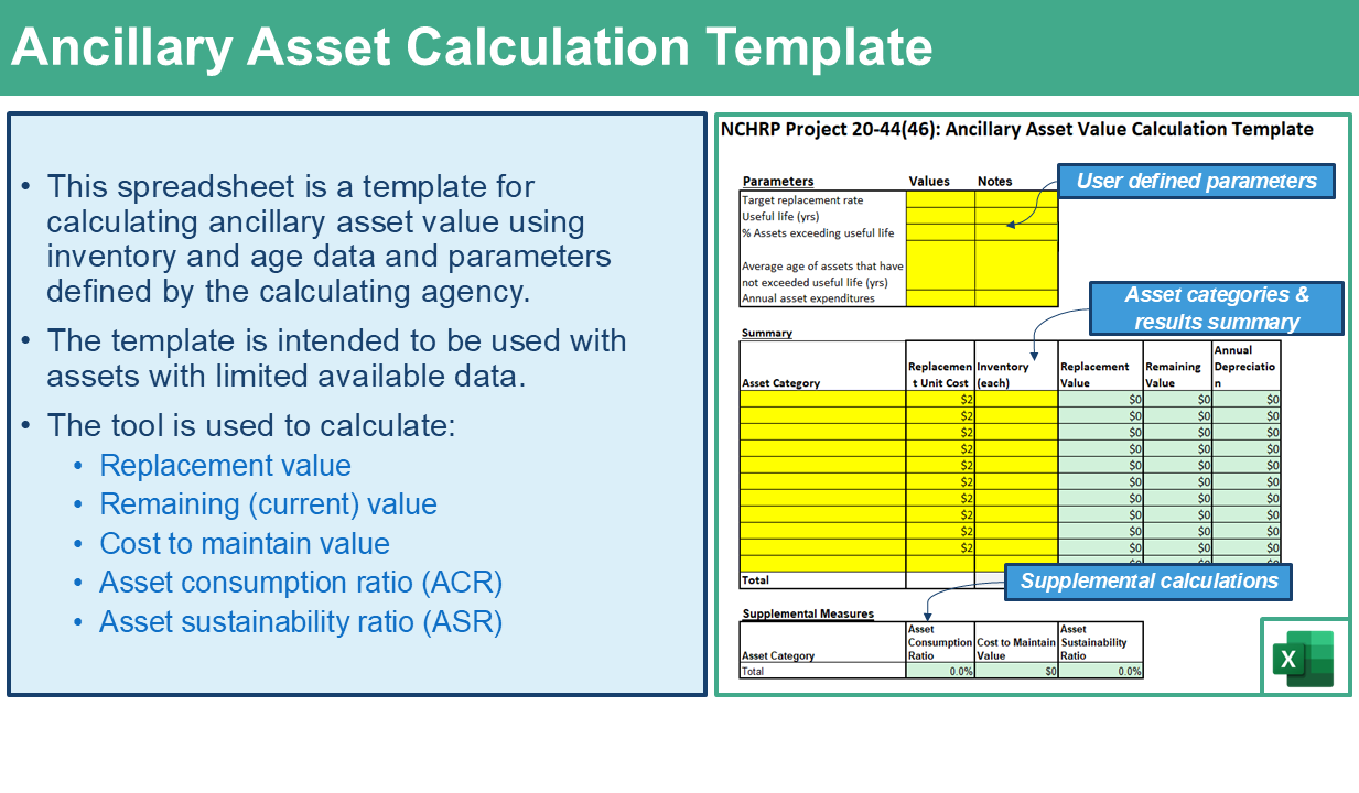
- Download the Ancillary Asset Calculation Template.
In this case study, a state department of transportation (DOT) located in the Northwest, labeled the “Northwestern DOT”, calculated asset value for its bridges using three depreciation approaches to measure their remaining (current) value. In comparing the results from the composite condition rating, minimum condition rating, and age-based approaches, the Northwestern DOT was able to gain a more complete understanding of its bridge inventory and identify the desired calculation approach for the agency’s needs.
Background
The Northwestern DOT’s primary driver for calculating and reporting asset value is to comply with the Federal Highway Administration’s (FHWA) requirement that State DOTs include a calculation of the value of National Highway System (NHS) pavement and bridge assets in their transportation asset management plans (TAMPs), and that they calculate the cost of maintaining asset value (23 CFR § 515.7(d)(4)).
In past versions of its TAMP, the Northwestern DOT estimated asset value based on replacement cost alone, without accounting for the assets’ age or condition. As a result, depreciation was not reflected in the valuation. This method also did not provide a useful estimate for the cost required to maintain asset value, since preserving full replacement value was calculated at $0. To enhance the accuracy and relevance of its asset valuations, the Northwestern DOT explored three depreciation-based approaches aimed at determining both the remaining value of bridges, and the cost necessary to sustain that value.
Methodology
Data
The Northwestern DOT used age and condition data from the National Bridge Inventory (NBI) to calculate asset value. For the age-based approach, each bridge’s value was calculated as a whole, while the condition-based approaches split each bridge into their three major components (deck, superstructure, substructure).
Condition-Based Approaches
While the relationship between the age of a bridge and its percent value remaining is assumed to be linear, bridges typically exhibit a non-linear relationship between condition and percent value remaining. The Northwestern DOT used data from a “do-nothing” scenario in the FHWA Bridge Investment Program (BIP) tool to develop deterioration curves for bridges within their jurisdiction based on component condition. The agency developed deterioration curves for each bridge component, as well as a “minimum component” deterioration curve based on the minimum component rating of a bridge. The end of life was defined as a component rating of 3.
Composite Component Rating Approach
The first approach tested by the Northwestern DOT was the composite component rating approach, in which the agency calculated the percent remaining value for each bridge component using the modeled deterioration curves. Those percentages were combined in a weighted average-based on defined parameters (20% deck, 40% superstructure, and 40% substructure) to obtain a composite percent value remaining for the entire bridge.
Minimum Component Rating Approach
The second approach was the minimum component rating approach, which used the lowest component condition rating of a bridge to define the effective age of the bridge.
Figure 9-10 shows the relationship between condition ratings and remaining value for each bridge component as well as for the minimum component. Note that the results shown for culverts are the same as that for substructure, as the agency found that culverts behaved similarly to substructures, but that there was not enough data for culverts to calculate a deterioration curve.
Age-Based Approach
The Northwestern DOT also used the typical bridge useful life to calculate an age-based valuation for each bridge. This method assumed linear depreciation by year, where the end of life for a bridge was set at 80 years and bridge age was defined by identifying the more recent of year built or year reconstructed. Figure 9-11 shows the curve representing the relationship between age and percent of value remaining for a given bridge.


Results
Table 9-12 summarizes the calculation of asset value for the Northwestern DOT’s bridges. The table includes replacement value as well as the remaining asset value based on the three approaches for calculating depreciation: using a weighted average of all three major components condition ratings, using the condition data of each bridge’s most degraded component, and using bridge age irrespective of condition. While the detailed results are available by owner (State DOT, Other), the case study results summarize all NBI bridges in the state, organized by whether or not the bridge is located on the National Highway System (On NHS, Off NHS).
Table 9-12. Asset Value Results
| NHS | Repl. Values ($B) | Remaining Asset Value by Method ($B) | ACR by Method (%) | Cost to Maintain by Method ($M) | ||||||
|---|---|---|---|---|---|---|---|---|---|---|
| Comp. Rating | Min. Rating | Age | Comp. Rating | Min. Rating | Age | Comp. Rating | Min. Rating | Age | ||
| State DOT | ||||||||||
| On | 45.3 | 34.1 | 29.6 | 22.5 | 75.3 | 65.3 | 49.6 | 871 | 1,118 | 552 |
| Off | 8.0 | 6.2 | 5.6 | 3.4 | 78.3 | 69.7 | 43.1 | 152 | 194 | 94 |
| Total | 53.3 | 40.3 | 35.1 | 25.9 | 75.8 | 66.0 | 48.6 | 1,023 | 1,313 | 646 |
| Other Owner | ||||||||||
| On | 5.6 | 4.1 | 3.5 | 2.9 | 73.4 | 64.0 | 53.0 | 107 | 138 | 61 |
| Off | 14.6 | 11.3 | 10.2 | 7.2 | 77.2 | 69.5 | 49.3 | 280 | 362 | 172 |
| Total | 20.2 | 15.4 | 13.7 | 10.2 | 76.2 | 68.0 | 50.3 | 387 | 500 | 233 |
| All | ||||||||||
| On | 50.8 | 38.2 | 33.1 | 25.4 | 75.1 | 65.2 | 50.0 | 978 | 1,256 | 613 |
| Off | 22.6 | 17.5 | 15.7 | 10.7 | 77.6 | 69.6 | 47.1 | 433 | 556 | 265 |
| Total | 73.4 | 55.7 | 48.9 | 36.1 | 75.9 | 66.5 | 49.1 | 1,410 | 1,812 | 878 |
Lessons Learned
Key takeaways from the Northwestern DOT’s comparison of age and condition-based depreciation approaches for bridge asset valuation are listed below:
- The approach chosen for calculating depreciation has a large impact on the end results. An agency should carefully consider which approach is most appropriate to meet its needs.
- The composite component condition approach typically yields a higher remaining value than the other approaches, as it considers the condition of each component of a bridge separately. This method accounts for the different characteristics of bridge components and allows the agency to adjust the weighting of each to match their standard practices.
- The minimum rating approach tends to yield lower valuations than the composite approach, as it uses the lowest component rating and assumes deterioration rates similar to that of the deck, typically the shortest-lived component. This approach also leads to a higher cost to maintain value compared to the composite approach, due to shorter useful life calculated in the model.
- Transportation agencies may select this approach to be conservative when calculating the value of their assets. Some bridge components are easier to repair or replace than others. For example, a bridge deck can be repaired or replaced relatively inexpensively, while a bridge substructure cannot be easily replaced without doing a full bridge construction.
- The age-based approach yields the lowest asset value, as it does not account for work performed on bridges to extend their life. A bridge that is beyond its useful life in age but has been well maintained and remains in good condition would have zero value remaining based purely on age.
- It is also essential that the parameters used in the calculations are consistent with the DOT’s real-world practices to get the most out of their calculation results.
- For example, the components in the composite approach should be weighted based on state-specific data and/or engineering judgement. Likewise, the definition of end of life should be aligned with current bridge management practices.
ACKNOWLEDGEMENT OF SPONSORSHIP
This work was sponsored by the American Association of State Highway and Transportation Officials, in cooperation with the Federal Highway Administration, and was conducted in the National Cooperative Highway Research Program (NCHRP), which is administered by the Transportation Research Board of the National Academies of Sciences, Engineering, and Medicine.
DISCLAIMER
This is an uncorrected draft as submitted by the research team.
This material is based upon work supported by the FHWA under Agreement No. 693JJ32350025. Any opinions, findings, and conclusions or recommendations expressed or implied in this document are those of the researchers who performed the research and are not necessarily those of the Transportation Research Board; the National Academies of Sciences, Engineering, and Medicine; the FHWA; or the program sponsors.
No warranty is made by the developers or their employer as to the accuracy, completeness, or reliability of this software and its associated equations and documentation. No responsibility is assumed by the developers for incorrect results or damages resulting from the use of this software.
COPYRIGHT
This material and the copyrights therein are owned by the National Academies of Sciences, Engineering, and Medicine.
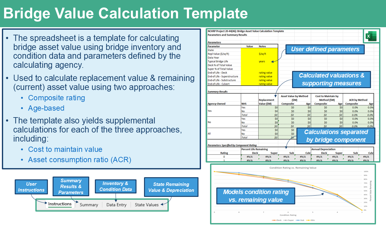
- Download the Bridge Value Calculation Template.
As part of NCHRP Project 20-44(46), the research team used data from the Federal Highway Administration’s (FHWA) Bridge Investment Program (BIP) tool to develop deterioration curves by component for bridges. The data includes all US states and offers a straightforward and repeatable approach to establishing a relationship between bridge condition and remaining value.
Background
Ideally calculations of bridge asset value should incorporate depreciation, or consumption of the value of a bridge asset. One approach for calculating depreciation is to observe a bridge’s current condition and then use a deterioration model to estimate the time until the bridge reaches its useful life. This analysis is typically performed by bridge component. Bridges typically have three components: the deck, superstructure and substructure, while bridge-length culverts have a single component, the culvert.
While all State DOTs have bridge management systems that can be used to estimate useful lives of bridge and culvert components, in practice the calculation can be cumbersome to perform. This case study provides an approach for making the depreciation calculation using state-specific data compiled by FHWA.
Data
The FHWA BIP is a competitive discretionary funding program for improving bridge condition as well as safety and reliability. The BIP includes data on expected deterioration for each bridge in the National Bridge Inventory (NBI). This was compiled by performing model runs in FHWA’s National Bridge Investment Analysis System (NBIAS). Data obtained from NBIAS to support the BIP includes predicted component ratings for each bridge and bridge-length culvert in the NBI over a fifty year time horizon, broken up into five year periods.
Methodology
The team defined the following process for using the data in the BIP to develop bridge component depreciation curves for a given state:
- The first step is to compile BIP data for the selected state. The BIP data detail the predicted time to deteriorate (in number of 5-year periods) from current conditions to each component condition and from the minimum component condition given no work is performed on the bridge.
- The next step is to calculate the average decline in component condition per period for each component for each bridge.
- Next it is necessary to calculate the average annual condition drop for each component by initial rating value (0-9). This is accomplished by weighting each bridge by deck area to account for size, and dividing the first (five year) period drop by five to get an annual average.
- The next step is to use the average annual condition drop to determine the average time required to deteriorate to each rating value starting from new condition.
- Finally the depreciation curve is calculated by establishing the percent of value remaining at each rating value for each component. This is calculated by subtracting from 100% the ratio of time to deteriorate to the rating value to the time to reach the end of life (e.g. a rating of 3).
In conjunction with bridge inventory data and unit cost data, the resulting deterioration curves can be used to calculate a remaining asset value.
Results
Figure 9-12 below provides an example calculation of the percentage of asset value remaining for each of the components of a bridge, as well as for the minimum component rating. As shown in the figure, a component is assumed to have reached the end of its useful life if its rating is 3 or less. The minimum component condition rating approach uses the lowest component condition rating to define the effective age of the bridge. Note this is an example set of curves: the process can be repeated to obtain state-specific curves.

Lessons Learned
Key takeaways from the development of an approach for developing bridge deterioration curves in support of asset valuation are listed below:
- When attempting to define the relationship between bridge condition and remaining value, observed deterioration curves can be developed using FHWA BIP data in the absence of readily available defined deterioration curves.
- State DOTs typically have existing bridge deterioration curves; however they may be embedded in management systems and difficult to extract, or a state may have many deterioration curves for families of bridges. The work described in the pilot offers a simplified approach to deriving deterioration curves for a state bridges by component, and thus a path toward calculating a depreciated current asset value.
- The approach should be adjusted to meet an agency’s needs and/or data.
- For example, a state may find that culverts behave similarly to substructures, but that there is not enough data for culverts to calculate the time to deteriorate to each rating value. In this case, it is acceptable to use a substitute curve, such as the one for substructures, to represent the relationship between culvert condition and remaining value.
ACKNOWLEDGEMENT OF SPONSORSHIP
This work was sponsored by the American Association of State Highway and Transportation Officials, in cooperation with the Federal Highway Administration, and was conducted in the National Cooperative Highway Research Program (NCHRP), which is administered by the Transportation Research Board of the National Academies of Sciences, Engineering, and Medicine.
DISCLAIMER
This is an uncorrected draft as submitted by the research team.
This material is based upon work supported by the FHWA under Agreement No. 693JJ32350025. Any opinions, findings, and conclusions or recommendations expressed or implied in this document are those of the researchers who performed the research and are not necessarily those of the Transportation Research Board; the National Academies of Sciences, Engineering, and Medicine; the FHWA; or the program sponsors.
No warranty is made by the developers or their employer as to the accuracy, completeness, or reliability of this software and its associated equations and documentation. No responsibility is assumed by the developers for incorrect results or damages resulting from the use of this software.
COPYRIGHT
This material and the copyrights therein are owned by the National Academies of Sciences, Engineering, and Medicine.
- Download the Bridge Value Calculation Template.
In this case study, a state-wide transportation agency in an eastern state, labeled the “Eastern DOT,” calculated the value of an existing bridge by determining the remaining user and social benefits of the structure. By comparing the anticipated lifecycle benefits with and without the bridge, Eastern DOT was able to determine the transportation and social value of the bridge to the traveling public and justify ongoing investments to keep it in good condition.
Background
Eastern DOT’s primary driver for calculating and reporting asset value is to comply with the Federal Highway Administration’s (FHWA) requirement that State DOTs include a calculation of the value of National Highway System (NHS) pavement and bridge assets in its transportation asset management plans (TAMPs). In prior TAMPs, Eastern DOT employed a condition-based depreciation approach based on replacement costs to understand and report asset values. However, this approach does not evaluate or communicate the value these assets provided to the public or the potential transportation or social loss that could result from failure to upkeep the assets. Eastern DOT decided to supplement its calculation methodology by testing an economic value-based approach for calculating the economic value of a bridge to the public.
Methodology
Data
Eastern DOT first determined traffic routing impacts in the absence of the bridge and then estimated future volumes and travel distances and times both with and without the facility. Starting with current volumes on the current and alternative routes, Eastern DOT computed the loss of demand due to congestion and assembled an inventory of travel times “with” and “without” the bridge. This inventory included motor vehicle traffic (car and light, medium, and heavy truck) and active transportation trips. The transportation data was supplemented with economic valuation estimates based on US Department of Transportation (USDOT) and Environmental Protection Agency (EPA) guidance.
Economic Value Approach
Eastern DOT assumed that the economic value equals the lifecycle benefits to users of having the asset in place and in good working condition. To determine these benefits, Eastern DOT calculated the travel time loss associated with the alternative routing required without the facility, including the loss to existing users of the replacement route who would face added congestion with additional traffic, the additional costs of operating vehicles along longer, more congested routes, the change in crashes expected due to the net change in vehicle-miles traveled (VMT) caused by the longer, slower route, changes in emissions, loss of mobility for those current trip makers who could be expected to avoid trip-making due to the longer, slower routing, and loss of bicycle trip access. There may be further disruptions or changes in the economy. These were not considered in the economic value approach, which focused only on the direct impacts.
Eastern DOT valued these impacts using USDOT and EPA estimates of travel time and costs, mobility value, costs of crashes by type, and the value of active transportation options. The net value of travel and emissions was calculated for both the “with” and “without” bridge cases over a thirty-year forecast. The future benefits were discounted based on USDOT guidance for an appropriate discount rate and then summed for each case. The Eastern DOT compared the total benefits of each case to estimate a loss that occurs in the “without” bridge case to determine its net present user and social value.
Results
Table 9-13 details the estimated user and social value by benefit category for both a current dollar and discounted dollar perspective. Consistent with USDOT guidance, the Eastern DOT applied a 3.1 percent discount rate, except for CO2 which was discounted at 2.0 percent (also per USDOT guidance). The discounted dollar estimate is the better economic value of the bridge.
Table 9-13. Asset User and Social Value Results
| Impact Category | Over the Project Lifecycle | |
|---|---|---|
| Constant Dollars | Discounted Dollars | |
| Costs of Additional Travel Time | $9,670.0 | $5,914.7 |
| Additional Vehicle Operating Costs | $846.4 | $522.9 |
| Safety Costs | $331.7 | $205.3 |
| Total Emission Costs | $153.6 | $109.6 |
| Loss of Mobility Value | $119.3 | $73.0 |
| Lost Bicycle Route Benefits | $0.01 | $0.007 |
| Total Bridge Value | $11,121.1 | $6,825.7 |
Lessons Learned
Lessons learned from the Eastern DOT’s experience in developing an economic value-based approach for bridge asset valuation include:
- Consideration of the travel impacts of the “without” case is crucial to understanding the facility valuation.
- The valuation approach applied utilizes speed-flow and elasticity of demand estimates to calculate future travel behavior.
- An approach utilizing a travel demand model might result in more defendable estimates.
- Economic valuation of assets is not widely understood but travel benefits are easily grasped by policy makers who intuitively understand the public benefits associated with their assets.
- As a result, an economic valuation is useful for justifying investments to maintain assets over a lifecycle.
- Future improvements to this case study could include using a travel demand model to estimate more precise rerouting travel impacts that may occur with and without the bridge.
- In addition, the estimated asset value reflects the operating conditions of the structure (e.g., traffic volumes and speeds experienced by users), but it does not consider asset deterioration. A variant of this approach could adjust the economic valuation using a measure of asset condition such as a bridge health index.
ACKNOWLEDGEMENT OF SPONSORSHIP
This work was sponsored by the American Association of State Highway and Transportation Officials, in cooperation with the Federal Highway Administration, and was conducted in the National Cooperative Highway Research Program (NCHRP), which is administered by the Transportation Research Board of the National Academies of Sciences, Engineering, and Medicine.
DISCLAIMER
This is an uncorrected draft as submitted by the research team.
This material is based upon work supported by the FHWA under Agreement No. 693JJ32350025. Any opinions, findings, and conclusions or recommendations expressed or implied in this document are those of the researchers who performed the research and are not necessarily those of the Transportation Research Board; the National Academies of Sciences, Engineering, and Medicine; the FHWA; or the program sponsors.
No warranty is made by the developers or their employer as to the accuracy, completeness, or reliability of this software and its associated equations and documentation. No responsibility is assumed by the developers for incorrect results or damages resulting from the use of this software.
COPYRIGHT
This material and the copyrights therein are owned by the National Academies of Sciences, Engineering, and Medicine.
In this case study, a metropolitan transportation agency, labeled the “Metropolitan TA,” calculated asset value for its pavements using a condition-based depreciation approach to calculate value. The agency was able to use calculated asset value to help justify on-going pavement maintenance investments.
Background
The Metropolitan TA’s primary driver for calculating and reporting asset value is to demonstrate the value of a targeted pavement investment program. The calculated asset value also is consistent with the Federal Highway Administration’s (FHWA) requirement for State DOTs to include a value of National Highway System (NHS) pavement and bridge assets in their transportation asset management plans (TAMPs), and that they calculate the cost of maintaining asset value (23 CFR § 515.7(d)(4)). The Metropolitan TA is interested in similar methodologies for its own TAMP.
In the Metropolitan TA’s previous TAMPs, asset value was calculated using a replacement cost approach that did not consider age or condition of the assets, and thus did not reflect depreciation of the assets. Also, the calculation did not yield a meaningful estimate of the cost to maintain asset value, since the cost to maintain replacement value was $0. The Metropolitan TA decided to improve its calculation methodology by testing a condition-based depreciation approach for calculating remaining asset value and the cost to maintain asset value.
Methodology
Data
The Metropolitan TA used a pavement condition index (PCI) based on pavement distress observations to categorize the condition of, and to manage its pavements, collected for each management section on the network. Pavement asset value was calculated for the pavement both on and off the NHS and then aggregated. Data was collected for 2017, 2019, 2021, and 2023 to support value trend analysis.
Condition-Based Value Approach
Asset value was assumed to depreciate relative to an estimated perfect condition value computed from cost to replace estimates specific to on- and off-NHS treatment requirements. This baseline value was computed for all pavements inclusive of bike lanes and parking areas. The PCI captured in the Metropolitan TA’s pavement inventory system was then used to depreciate the value to a condition-based value. This exercise was repeated for each year of the analysis to assess trends in valuation. Then a cost to improve to full value was estimated to compare the valuation trend to the condition-based valuation.
The Metropolitan TA used valuation estimates to assess the impact of its pavement condition investment program. In addition, the agency calculated a cost to improve value across the whole of the network. The calculations were performed in a spreadsheet tool where the agency could adjust parameters (e.g. cost to improve and maintain) to see the impact on the results.
Results
Table 9-14 details the calculation of the current condition-based asset value for the Metropolitan TA’s pavements. The table shows replacement value and remaining asset value based on the PCI estimate as well as the cost to maintain based on PCI-specific treatment costs for on- and off-NHS pavements. The results are summarized by pavement location relative to the National Highway System (On NHS, Off NHS).
Table 9-14. Asset Value Results
| NHS | Replacement Value ($M) | Remaining Asset Value by PCI Method ($M) | Cost to Maintain ($M) |
|---|---|---|---|
| On | $707.3 | $624.4 | $26.2 |
| Off | $2,536.9 | $1,951.3 | $219.6 |
| Total | $3,244.2 | $2,575.8 | $245.8 |
Lessons Learned
Lessons learned from the Metropolitan TA’s experience in developing a condition-based depreciation approach to pavement asset valuation include:
- Using condition-based depreciation approach is useful for justifying an investment in condition improvement and for assessing valuation over time.
- The valuation approach sets alternatives for asset maintenance on a common valuation system and is useful for communicating the scale of both value and potential loss when determining an investment strategy.
- A time-based comparison of valuations mixes deterioration and improvement in a way that can be challenging to communicate unless carefully delineated.
- The cost-to-maintain parameter has a significant impact on the results. Costs change over time and retrospective analysis should consider the impact of both practice and inflation over time. Future valuation should be adjusted as needed.
- Future enhancements could include comparisons of the change in asset valuations to the investments in the pavement program, while considering the yearly deterioration in pavement condition.
ACKNOWLEDGEMENT OF SPONSORSHIP
This work was sponsored by the American Association of State Highway and Transportation Officials, in cooperation with the Federal Highway Administration, and was conducted in the National Cooperative Highway Research Program (NCHRP), which is administered by the Transportation Research Board of the National Academies of Sciences, Engineering, and Medicine.
DISCLAIMER
This is an uncorrected draft as submitted by the research team.
This material is based upon work supported by the FHWA under Agreement No. 693JJ32350025. Any opinions, findings, and conclusions or recommendations expressed or implied in this document are those of the researchers who performed the research and are not necessarily those of the Transportation Research Board; the National Academies of Sciences, Engineering, and Medicine; the FHWA; or the program sponsors.
No warranty is made by the developers or their employer as to the accuracy, completeness, or reliability of this software and its associated equations and documentation. No responsibility is assumed by the developers for incorrect results or damages resulting from the use of this software.
COPYRIGHT
This material and the copyrights therein are owned by the National Academies of Sciences, Engineering, and Medicine.
In this case study, the research team calculated developed a depreciation curve for cutaway buses using the market perspective to estimate current asset value. In comparing the results obtained using market value with those obtained by applying a linear, age-based depreciation curve to replacement value, the research team found the market value provides a different, and potentially more accurate calculation of asset value.
Background
Calculations of asset value should ideally incorporate depreciation, or consumption of the value of an asset. Where a market exists for resale of an asset the effect of depreciation is directly measurable: it is the difference between the purchase price of a new asset and the resale value of a used one. Where no such market exists it is necessary to calculate depreciation through other means. The most straightforward approach for doing so it to establish the useful life of an asset and then assume straight-line depreciation as a function of age.
This case study provides an example of how the market value can be used to help establish asset value. In this example the research team established market values for used assets for a particular asset class, cutaway buses, and then derived a depreciation curve from the market data.
Methodology
Data
In its National Transit Database (NTD) the Federal Transit Administration (FTA) defines a “cutaway bus” as “A vehicle in which a bus body is mounted on the chassis of a van or light-duty truck. The original van or light-duty truck chassis may be reinforced or extended. Cutaways typically seat 15 or more passengers, and typically may accommodate some standing passengers…” (61) In the U.S. thousands of transit agencies rely on cutaways for transit and paratransit service. As shown in Table 9-15, FTA estimates that the useful life of a cutaway is approximately 10 years. (62)
Table 9-15. Default Useful Life Benchmarks for Transit Vehicles
| Vehicle Type | Default ULB (years) | Vehicle Type | Default ULB (years) |
|---|---|---|---|
| Articulated bus | 14 | Minivan | 8 |
| Automated guideway vehicle | 31 | Commuter rail locomotive | 39 |
| Automobile | 8 | Commuter rail passenger coach | 39 |
| Over-the-road bus | 14 | Commuter rail self-propelled passenger car | 39 |
| Bus | 14 | School bus | 14 |
| Cable car | 112 | Steel wheel vehicles | 25 |
| Cutaway bus | 10 | Streetcar | 31 |
| Double decked bus | 14 | Sport utility vehicle | 8 |
| Ferryboat | 42 | Trolleybus | 13 |
| Heavy rail passenger car | 31 | Trucks and other rubber tire vehicles | 14 |
| Inclined plane vehicle | 56 | Aerial tramway | 12 |
| Light rail vehicle | 31 | Van | 8 |
| Monorail vehicle | 31 | Vintage trolley | 58 |
Given the large inventory of cutaway vehicles, and the fact that a vehicle may be readily transferred from one owner to another, a well-defined market exists for resale of cutaway buses. Thus, the research team selected the cutaway bus as an example asset to use to illustrate calculation of asset value using a market perspective.
To establish market value for cutaways the team first selected a common cutaway configuration, specifically cutaways configured for passenger service using a Ford E450 chassis. The research team then queried six different publicly-available systems for resale of vehicles. Four of the six systems list prices for vehicles, and two offer vehicles for auction. For the auction-based systems the team relied on completed sales rather than requested prices. Figure 1 is a scatter plot of showing prices as a function of vehicle age established in this step. As illustrated in the figure, data were collected for 34 vehicles that range in age from 0 to 11 years. Prices were found vary from $4,650 to $142,725. The team tested the correlation between price and both age and mileage, but found a stronger correlation between price and age than between price and mileage.

Depreciation Curve Development
The team next calculated a depreciation curve for cutaway vehicles by fitting an exponential curve to the data. The equation of the curve showing the relationship between age and price is as follows:
P(t) = ae^{bt}
Where P is the price of a vehicle with age t and a and b are parameters fit from the data. The best-fit curve has an R-squared value of 0.81, which indicates a reasonable correlation between the age and price.
The resulting curve predicts market value as a function of age. The curve may be restated to predict value as a percent of new vehicle cost by dividing all values by the parameter a (calculated as $132,701 for this data set). The equation of the best-fit curve recast in this fashion is:
V(t) = e^{-0.204t}
Where V is the remaining value as a percent of a new vehicle cost at age t.
The research team also calculated a simplified depreciation curve assuming straight-line depreciation from 0 to 10 years. Figure 2 shows the two alternative depreciation curves. Compared to the straight-line depreciation approach, the best-fit curve fit based on market values shows accelerated depreciation for ages less than eight years. This behavior is consistent with typical vehicle pricing on the open market experienced by consumers: a new vehicle loses value quickly after its purchase, but holds some value for a number of years.

Illustrative Example
As an illustration of the approach, assume there is a transit agency with a fleet of cutaways evenly distributed in age from 0 to 10 years. In this fleet, the average age of a cutaway would be 5 years. Using the linear depreciation approach, the average remaining value of a vehicle would be 50% of the value of a new vehicle based on the assumption of straight-line depreciation. By contrast, based on market value the average remaining value would be 44% of the value of a new vehicle. This result may be obtained by calculating value for each age from 0 to 10 years and averaging the result. Thus, in this case using market value results in value that is approximately 12% lower than that estimated using straight-line depreciation.
However, if the fleet of cutaways had an even age distribution between 6 and 14 years, the average remaining value of a vehicle would be calculated as approximately 11% of new vehicle cost using straight-line depreciation and 15% using market value. In this case, the market value depreciation curve yields a higher remaining value for the vehicles. A summary of example scenarios is included in Table 9-16.
Table 9-16. Example Applications of Market Value and Linear Depreciation Approaches
| Fleet Age Distribution (years) | Vehicle Unit Repl. Value ($) | Market Value Approach | Linear Depreciation Approach | ||
|---|---|---|---|---|---|
| Avg. Remaining Value by Vehicle ($) | Avg. Remaining Value by Vehicle (%) | Avg. Remaining Value by Vehicle (%) | Avg. Remaining Value by Vehicle (%) | ||
| 0 to 10 | 132,701 | $58,441 | 44% | $66,351 | 50% |
| 6 to 14 | $19,748 | 15% | $14,745 | 11% | |
Lessons Learned
Conclusions drawn from this case study include the following:
- For an asset for which a market exists, it is possible to calculate depreciation using the market perspective.
- Calculating asset value using the market perspective can be a challenge for many transportation assets because a market for resale of culverts, overhead signs, bridges, and guardrail hardly exists. However, in the case where a market does exist, such as for vehicles, asset price data from sales on the open market can be used to develop a depreciation curve for a given asset.
- The depreciation curve resulting from the market perspective may differ significantly from a simple linear depreciation approach.
- A vehicles price on the market theoretically represents all the available information about the asset, such as any treatments performed on the asset and the condition of the asset. Thus the vehicles price may better represent the remaining value than its age, particularly as a vehicle approaches its typical useful life. A depreciation curve based on market values may yield higher remaining value for older vehicles relative to a straight-line depreciation approach, while the opposite may be true for newer vehicles.
ACKNOWLEDGEMENT OF SPONSORSHIP
This work was sponsored by the American Association of State Highway and Transportation Officials, in cooperation with the Federal Highway Administration, and was conducted in the National Cooperative Highway Research Program (NCHRP), which is administered by the Transportation Research Board of the National Academies of Sciences, Engineering, and Medicine.
DISCLAIMER
This is an uncorrected draft as submitted by the research team.
This material is based upon work supported by the FHWA under Agreement No. 693JJ32350025. Any opinions, findings, and conclusions or recommendations expressed or implied in this document are those of the researchers who performed the research and are not necessarily those of the Transportation Research Board; the National Academies of Sciences, Engineering, and Medicine; the FHWA; or the program sponsors.
No warranty is made by the developers or their employer as to the accuracy, completeness, or reliability of this software and its associated equations and documentation. No responsibility is assumed by the developers for incorrect results or damages resulting from the use of this software.
COPYRIGHT
This material and the copyrights therein are owned by the National Academies of Sciences, Engineering, and Medicine.
In this case study, the state department of transportation in a Western state, labeled “Western DOT,” calculated the value of an existing highway by determining the remaining user and social benefits of the facility. By comparing the anticipated lifecycle benefits with and without the highway, Western DOT was able to determine the transportation and social value the highway provides to the traveling public and businesses, helping to justify ongoing investments to keep it in good condition.
Background
Western DOT’s primary driver for calculating and reporting asset value was to comply with the Federal Highway Administration’s (FHWA’s) requirement that State DOTs include a calculation of the value of National Highway System (NHS) pavement and bridge assets in its transportation asset management plan (TAMP). In prior TAMPs, Western DOT employed a straight-line depreciation approach based on investment costs to understand and report asset values. However, this approach does not evaluate or communicate the value these assets provide to the public or the potential transportation or social loss that could result from failure to upkeep their assets. The highway selected for evaluation is a significant freight corridor and failure to upkeep would likely carry economic consequences beyond the vehicles and drivers on the road. The value to the economy is not captured under their traditional approach to asset valuation. Western DOT decided to supplement its calculation methodology by testing an economic value-based approach to estimate the highway’s economic value to the public.
Methodology
Data
Western DOT first determined freight and passenger traffic routing impacts in the absence of the highway and then estimated future volumes, travel time and distances both with and without the facility. Starting with current volumes derived from weigh station counts on both the existing and alternative routes and modes, Western DOT computed mode shifts and loss of demand due to changes in travel time and costs and assembled a comparative inventory of travel times “with” and “without” the highway. This inventory included freight motor vehicle traffic, personal vehicle traffic, and freight movements associated with non-highway modes. The transportation data was supplemented with economic valuation estimates based on US Department of Transportation (USDOT), Western DOT studies, public data on freight movement costs and times, and US Department of Energy (US DOE) guidance.
Economic Value Approach
Western DOT assumed that the highway’s economic value corresponds to the lifecycle benefits it provides to users and freight shippers when the asset is in place and maintained in good working condition. To determine these benefits, Western DOT calculated the travel time loss and additional costs associated with the alternative routing required without the facility. Additionally, Western DOT considered increased costs to shippers associated with quicker but more costly shipping times, changes in crash rates due to the net change in vehicle-miles traveled (VMT) as a result of the anticipated freight mode shifts and personal travel trip making reductions, changes in emissions, loss of mobility for current trip makers who could be expected to avoid trip-making due to the loss of access. There may be further disruptions or changes in the economy. These were not considered in the economic value approach, which focused only on the direct impacts.
Western DOT valued these impacts using USDOT and EPA estimates of travel time and costs, data on the economic cost of delay in freight movements from the academic literature, costs of crashes by type, and the value of GHG emissions. The net value of travel and emissions was calculated for both the “with” and “without” highway scenarios over a thirty-year forecast. The future benefits were discounted based on USDOT guidance for an appropriate discount rate and then summed for each case. The Western DOT compared the total benefits of each case to estimate a loss that occurs in the “without” highway case to determine its net present user and social value.
Results
Table 9-17 details the estimated user and social value by benefit category for both a current dollar and discounted dollar perspective. Consistent with USDOT’s 2024 guidance, the Western DOT applied a 3.1 percent discount rate, except for CO2 which was discounted at 2.0 percent (also per USDOT guidance). The discounted dollar estimate is the better economic value of the highway.
Table 9-17. Asset User and Social Value Results, in millions
| Impact Category | Over a 30-Year Project Lifecycle | |
|---|---|---|
| Constant Dollars | Discounted at 3.1% | |
| Costs of Additional Travel Time | $2,768.6 | $1,729.1 |
| Additional Vehicle Operating Costs | $23,732.7 | $14,821.7 |
| Commodity Delay Cost | -$10,370.9 | -$6,479.9 |
| Total Emission (GHG) Costs | $16,009.1 | $11,454.5 |
| Safety Costs | -$342.8 | -$214.5 |
| Total Benefits | $31,789.5 | $21,306.5 |
Lessons Learned
Lessons learned from the Western DOT’s experience in developing an economic value-based approach for highway asset valuation include:
- For freight corridors, it is essential to consider not only alternative routes, but also alternative modes of transport, assuming that shippers will find a way to move freight regardless of cost.
- For alternative freight modes, there can be a trade-off between time and cost, and both need consideration in order to accurately quantify the net value of the facility.
- Shippers’ behavior in the absence of the highway was estimated for this case study based on data from before the opening of the highway, but also from data covering a prior closure due to flooding.
- Prior event data can be useful for estimating behavior in an alternative scenario.
- Future improvements to this case study could include using a multi-modal travel demand model to estimate more precisely the rerouting travel impacts that may occur with and without the highway
- This might also include a consideration of emerging freight delivery technologies (such as drones and pilotless aircraft) and their impact on the decision making for rerouting.
- Economic valuation of assets is not widely understood but travel benefits are easily grasped by policy makers who intuitively understand the public benefits associated with their assets.
- As a result, an economic valuation is useful for justifying investments to maintain assets over a lifecycle.
- In addition, the estimated asset value reflects the operating conditions of the structure (e.g., traffic volumes and speeds experienced by users), but it does not consider asset deterioration. A variant of this approach could adjust the economic valuation using a measure of asset condition such as a pavement condition index.
ACKNOWLEDGEMENT OF SPONSORSHIP
This work was sponsored by the American Association of State Highway and Transportation Officials, in cooperation with the Federal Highway Administration, and was conducted in the National Cooperative Highway Research Program (NCHRP), which is administered by the Transportation Research Board of the National Academies of Sciences, Engineering, and Medicine.
DISCLAIMER
This is an uncorrected draft as submitted by the research team.
This material is based upon work supported by the FHWA under Agreement No. 693JJ32350025. Any opinions, findings, and conclusions or recommendations expressed or implied in this document are those of the researchers who performed the research and are not necessarily those of the Transportation Research Board; the National Academies of Sciences, Engineering, and Medicine; the FHWA; or the program sponsors.
No warranty is made by the developers or their employer as to the accuracy, completeness, or reliability of this software and its associated equations and documentation. No responsibility is assumed by the developers for incorrect results or damages resulting from the use of this software.
COPYRIGHT
This material and the copyrights therein are owned by the National Academies of Sciences, Engineering, and Medicine.
This section describes cases studies profiling the asset valuation approaches of two highway agencies from Britain and Australia. Each case study demonstrates how the agency defines its asset hierarchy, establishes replacement costs, and calculates depreciation. The agencies profiled in the case studies follow the asset valuation guidance established in their respective countries, and their work in this area predates the development of this document. Nonetheless, both agencies use approaches that are very consistent with the guidance presented here, illustrating the common philosophy between the guidance, international standards for calculating asset value, and the state of the practice worldwide.
Highways England
Highways England is a public company responsible for managing the Strategic Road Network (SRN) in England, which is a core set of 4,300 miles of major roads that represents a third of all road traffic and two thirds of freight traffic. The organization is wholly owned by the British government and receives all of its capital and revenue funding directly from the United Kingdom (UK) Department for Transport (DfT). Nonetheless, Highways England operates as a company, and produces company financial accounts to provide visibility of its ongoing stewardship and value in terms of taxpayer equity. Asset value is computed and reported as part of the organization’s financial health.
The following paragraphs describe the approach used by Highways England to value its portion of the total British SRN. Note that Highway England’s approach is also used by the other SRN operating organizations: Transport Scotland for the SRN in Scotland; the Welsh Government for the SRN in Wales; and the Northern Ireland Department for Infrastructure for the SRN and all local roads in Northern Ireland. Additionally, the Northern Ireland Department for Infrastructure uses the same methodology for river and coastal assets in Northern Ireland.
Highways England’s approach to asset valuation is undertaken in accordance with Government Financial Reporting Manual (FReM) (49). For infrastructure assets, the manual uses the principles of Royal Institution of Chartered Surveyors (RICS) as described in the RICS “Red Book” (50). The company determines the fair value of the SRN using Depreciated Replacement Cost (DRC) in accordance with the guidance provided by the FReM and the Red Book. This approach is consistent with accounting standard IFRS 13 for calculating fair value (3). It results in the calculation of the value of the SRN from the perspective of a theoretical buyer based on how much it would cost to construct a network of equivalent service potential.
Figure 9-15 summarizes the process used by Highways England for calculating value. First, the organization calculates capital expenses. These costs are adjusted to obtain the ‘as new’ replacement cost based on a modern equivalent asset offering the same function (which the company establishes as identical routing and capacity) on a greenfield site.
Replacement costs are calculated for four asset classes:
- Pavements;
- Structures;
- Technology Assets; and
- Land
Note that the valuation for pavement is assumed to include the value of a number of other ancillary assets, such as vehicle restraint systems, signage, drainage, and other traffic and safety assets. For each asset class Highways England first calculates unit rates, and then applies the unit rate to the asset quantity to calculate replacement cost.
Following the calculation of replacement cost, the organization then calculates depreciation. Depreciation and other adjustments account for impaired or obsolete (derecognized) assets and are applied to the replacement cost to obtain DRC. Depreciation of asset value is calculated based upon asset condition surveys. While renewals are performed that improve conditions, these are not treated for accounting purposes as having an impact upon the valuation of the network because any related improvement in road condition are reflected in the condition surveys. Thus, Highways England depreciate 100% of renewals expenditures in the year that they are incurred.

Depreciation is based on the observed condition of assets. For pavement, condition is measured based on rutting. For structures, an Element Condition Score is obtained from structure inspections performed for each element of a structure. Land assets are not depreciated.
To ensure a robust valuation, Highways England undertakes a full valuation of each asset category at intervals not exceeding five years. A revaluation of pavements and lands was undertaken in the period of 2019 to 2020. At the time of that valuation, the value of the SRN was estimated to be approximately £123.2 billion. Updated valuations of structures and technology are planned in 2023 and 2024, respectively.
Highways England makes improvements to its valuation approach on a continuing basis. For example, historically depreciation for pavement is calculated based on rutting. In the future, Highways England plans to improve this depreciation calculation by including other pavement distresses, such as fretting, texture, and longitudinal cracking. Also, the organization plans to perform a separate calculation for special structures, unique to the network, that are best valued on a case-by-case basis rather than using unit rates.
Australian Road Authority
This case study describes the asset valuation approach used by a major government road authority in Australia. The authority is responsible for managing a large network of public roads, privately-funded toll roads, bridges, culverts, tunnels, and other assets. Valuations are conducted according to local government and national (Australian) accounting policies and standards. These standards emphasize basing estimates on fair value, consistent with international accounting standards.
The agency uses what it calls “Optimized Depreciated Replacement Cost (ODRC)” to value its assets. This term highlights that the replacement cost used is the cost to replace an asset with its modern equivalent, rather than the cost of a replacing an asset in-kind.
Figure 9-16 summarizes the process used by the authority to calculate fair value for its assets. As shown in the figure, the process includes steps for calculating replacement cost, and then adjusting replacement cost based on deprecation. Note the authority’s process includes some additional steps not shown in the figure which further modify fair value to reflect planned work.

The approach is applied to calculate value for four asset classes: roads; minor roads; bridges; and tunnels. Assets are valued at the component-level where sufficient data are available to support the calculation. Figure 9-17 shows how roads and bridges are subdivided into components.

Depreciation is calculated based on condition data where data are available to support the calculation. For example, the authority calculates a measure of pavement condition called Pavement Health Index (PHI) which is based on data for rutting, cracking, and other pavement distresses. Separately the authority performs an analysis to relate PHI to effective age. This relationship is applied to estimate the effective age of each segment, which is subsequently used to calculate depreciation for the pavement wearing surface. Figure 9-18 shows the relationship between PHI and effective age for flexible pavement.
Note that where detailed data are unavailable for a given asset component, the value of the component is estimated as a percentage of the value of the asset. Also, earthwork assets are not depreciated.
The end result of the calculation is an asset value that is comprehensive, leverages detailed data on individual components, and reflects best engineering judgement on asset condition and remaining life.
