In this case study, the research team calculated developed a depreciation curve for cutaway buses using the market perspective to estimate current asset value. In comparing the results obtained using market value with those obtained by applying a linear, age-based depreciation curve to replacement value, the research team found the market value provides a different, and potentially more accurate calculation of asset value.
Background
Calculations of asset value should ideally incorporate depreciation, or consumption of the value of an asset. Where a market exists for resale of an asset the effect of depreciation is directly measurable: it is the difference between the purchase price of a new asset and the resale value of a used one. Where no such market exists it is necessary to calculate depreciation through other means. The most straightforward approach for doing so it to establish the useful life of an asset and then assume straight-line depreciation as a function of age.
This case study provides an example of how the market value can be used to help establish asset value. In this example the research team established market values for used assets for a particular asset class, cutaway buses, and then derived a depreciation curve from the market data.
Methodology
Data
In its National Transit Database (NTD) the Federal Transit Administration (FTA) defines a “cutaway bus” as “A vehicle in which a bus body is mounted on the chassis of a van or light-duty truck. The original van or light-duty truck chassis may be reinforced or extended. Cutaways typically seat 15 or more passengers, and typically may accommodate some standing passengers…” (61) In the U.S. thousands of transit agencies rely on cutaways for transit and paratransit service. As shown in Table 9-15, FTA estimates that the useful life of a cutaway is approximately 10 years. (62)
Table 9-15. Default Useful Life Benchmarks for Transit Vehicles
| Vehicle Type | Default ULB (years) | Vehicle Type | Default ULB (years) |
|---|---|---|---|
| Articulated bus | 14 | Minivan | 8 |
| Automated guideway vehicle | 31 | Commuter rail locomotive | 39 |
| Automobile | 8 | Commuter rail passenger coach | 39 |
| Over-the-road bus | 14 | Commuter rail self-propelled passenger car | 39 |
| Bus | 14 | School bus | 14 |
| Cable car | 112 | Steel wheel vehicles | 25 |
| Cutaway bus | 10 | Streetcar | 31 |
| Double decked bus | 14 | Sport utility vehicle | 8 |
| Ferryboat | 42 | Trolleybus | 13 |
| Heavy rail passenger car | 31 | Trucks and other rubber tire vehicles | 14 |
| Inclined plane vehicle | 56 | Aerial tramway | 12 |
| Light rail vehicle | 31 | Van | 8 |
| Monorail vehicle | 31 | Vintage trolley | 58 |
Given the large inventory of cutaway vehicles, and the fact that a vehicle may be readily transferred from one owner to another, a well-defined market exists for resale of cutaway buses. Thus, the research team selected the cutaway bus as an example asset to use to illustrate calculation of asset value using a market perspective.
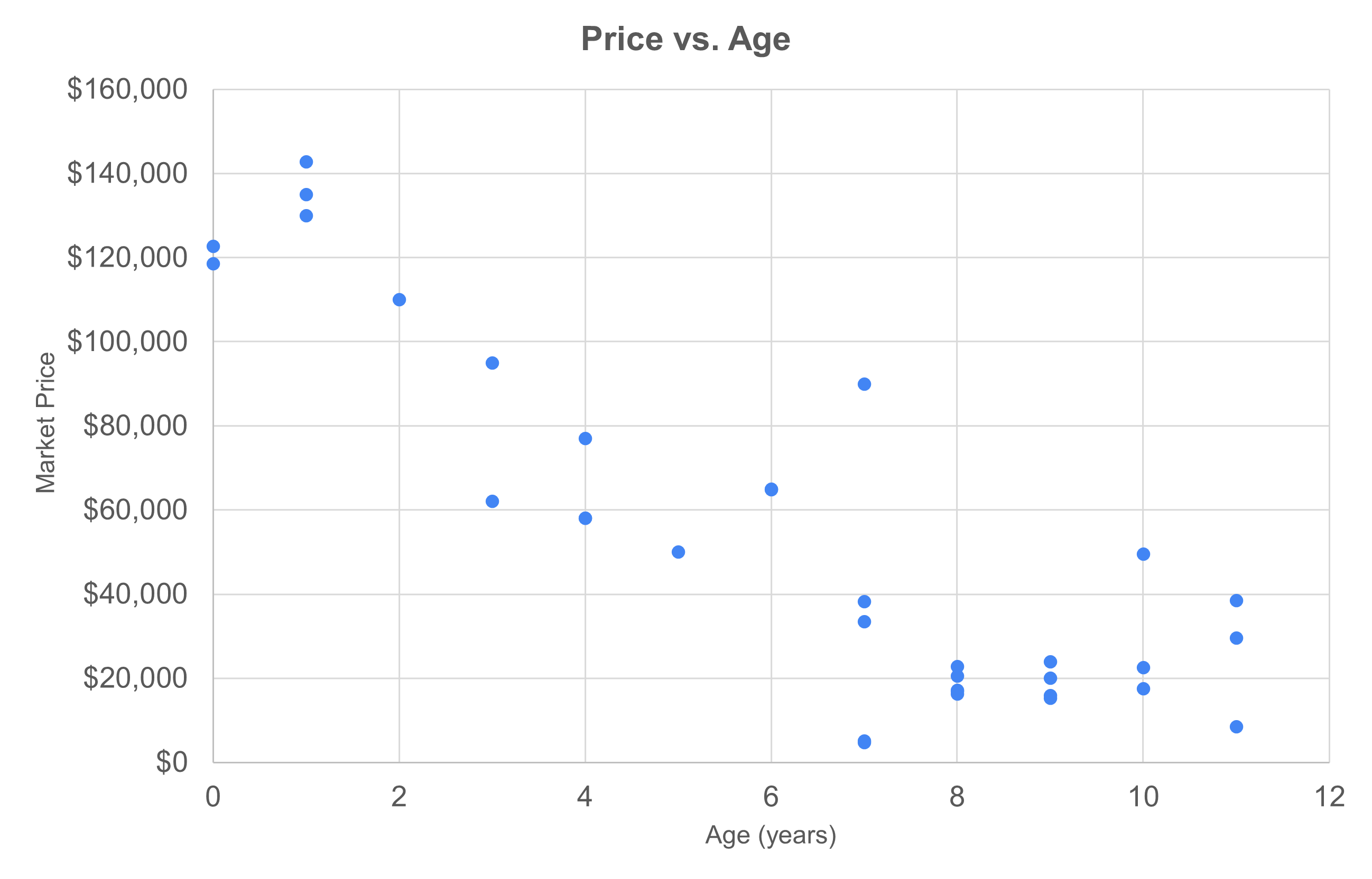
To establish market value for cutaways the team first selected a common cutaway configuration, specifically cutaways configured for passenger service using a Ford E450 chassis. The research team then queried six different publicly-available systems for resale of vehicles. Four of the six systems list prices for vehicles, and two offer vehicles for auction. For the auction-based systems the team relied on completed sales rather than requested prices. Figure 1 is a scatter plot of showing prices as a function of vehicle age established in this step. As illustrated in the figure, data were collected for 34 vehicles that range in age from 0 to 11 years. Prices were found vary from $4,650 to $142,725. The team tested the correlation between price and both age and mileage, but found a stronger correlation between price and age than between price and mileage.
Depreciation Curve Development
The team next calculated a depreciation curve for cutaway vehicles by fitting an exponential curve to the data. The equation of the curve showing the relationship between age and price is as follows:
P(t) = ae^{bt}
Where P is the price of a vehicle with age t and a and b are parameters fit from the data. The best-fit curve has an R-squared value of 0.81, which indicates a reasonable correlation between the age and price.
The resulting curve predicts market value as a function of age. The curve may be restated to predict value as a percent of new vehicle cost by dividing all values by the parameter a (calculated as $132,701 for this data set). The equation of the best-fit curve recast in this fashion is:
V(t) = e^{-0.204t}
Where V is the remaining value as a percent of a new vehicle cost at age t.
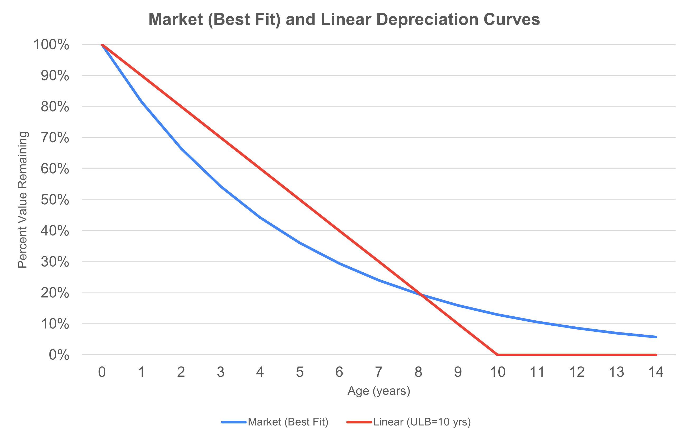
The research team also calculated a simplified depreciation curve assuming straight-line depreciation from 0 to 10 years. Figure 2 shows the two alternative depreciation curves. Compared to the straight-line depreciation approach, the best-fit curve fit based on market values shows accelerated depreciation for ages less than eight years. This behavior is consistent with typical vehicle pricing on the open market experienced by consumers: a new vehicle loses value quickly after its purchase, but holds some value for a number of years.
Illustrative Example
As an illustration of the approach, assume there is a transit agency with a fleet of cutaways evenly distributed in age from 0 to 10 years. In this fleet, the average age of a cutaway would be 5 years. Using the linear depreciation approach, the average remaining value of a vehicle would be 50% of the value of a new vehicle based on the assumption of straight-line depreciation. By contrast, based on market value the average remaining value would be 44% of the value of a new vehicle. This result may be obtained by calculating value for each age from 0 to 10 years and averaging the result. Thus, in this case using market value results in value that is approximately 12% lower than that estimated using straight-line depreciation.
However, if the fleet of cutaways had an even age distribution between 6 and 14 years, the average remaining value of a vehicle would be calculated as approximately 11% of new vehicle cost using straight-line depreciation and 15% using market value. In this case, the market value depreciation curve yields a higher remaining value for the vehicles. A summary of example scenarios is included in Table 9-16.
Table 9-16. Example Applications of Market Value and Linear Depreciation Approaches
| Fleet Age Distribution (years) | Vehicle Unit Repl. Value ($) | Market Value Approach | Linear Depreciation Approach | ||
|---|---|---|---|---|---|
| Avg. Remaining Value by Vehicle ($) | Avg. Remaining Value by Vehicle (%) | Avg. Remaining Value by Vehicle (%) | Avg. Remaining Value by Vehicle (%) | ||
| 0 to 10 | 132,701 | $58,441 | 44% | $66,351 | 50% |
| 6 to 14 | $19,748 | 15% | $14,745 | 11% | |
Lessons Learned
Conclusions drawn from this case study include the following:
- For an asset for which a market exists, it is possible to calculate depreciation using the market perspective.
- Calculating asset value using the market perspective can be a challenge for many transportation assets because a market for resale of culverts, overhead signs, bridges, and guardrail hardly exists. However, in the case where a market does exist, such as for vehicles, asset price data from sales on the open market can be used to develop a depreciation curve for a given asset.
- The depreciation curve resulting from the market perspective may differ significantly from a simple linear depreciation approach.
- A vehicles price on the market theoretically represents all the available information about the asset, such as any treatments performed on the asset and the condition of the asset. Thus the vehicles price may better represent the remaining value than its age, particularly as a vehicle approaches its typical useful life. A depreciation curve based on market values may yield higher remaining value for older vehicles relative to a straight-line depreciation approach, while the opposite may be true for newer vehicles.
ACKNOWLEDGEMENT OF SPONSORSHIP
This work was sponsored by the American Association of State Highway and Transportation Officials, in cooperation with the Federal Highway Administration, and was conducted in the National Cooperative Highway Research Program (NCHRP), which is administered by the Transportation Research Board of the National Academies of Sciences, Engineering, and Medicine.
DISCLAIMER
This is an uncorrected draft as submitted by the research team.
This material is based upon work supported by the FHWA under Agreement No. 693JJ32350025. Any opinions, findings, and conclusions or recommendations expressed or implied in this document are those of the researchers who performed the research and are not necessarily those of the Transportation Research Board; the National Academies of Sciences, Engineering, and Medicine; the FHWA; or the program sponsors.
No warranty is made by the developers or their employer as to the accuracy, completeness, or reliability of this software and its associated equations and documentation. No responsibility is assumed by the developers for incorrect results or damages resulting from the use of this software.
COPYRIGHT
This material and the copyrights therein are owned by the National Academies of Sciences, Engineering, and Medicine.

